Extreme value theory and peaks over threshold model in the Russian stock market

quantile of the distribution of losses (for example the 95th percentile): VaR_p=F ' (p) , where F is the loss cumulative distribution function and p the selected probability level. Traditional procedure calculating VaR based on normal distribution has limitations. VaR model reflects that it is to asses the possible maximum loss under regular market environments. Risk managers have become more concerned with events occurring under extreme market conditions [2,3]. This paper argues that extreme value theory (EVT) and POT (Peaks Over Threshold) model provide tools for estimating measures of tail risk under irregular volatility in market. We consider a fully parametric model, based on the GPD (Generalized Pareto Distribution), which can be easily estimated by maximum likelihood method [4,5].

I.    Theoretical framework of the extreme value approach

Extreme value theory is a powerful and fairly robust framework to study the tail behavior of a distribution. There have been a number of extreme value studies in the finance literature in recent years: quantile estimation using the extreme value theory [6]; the estimation of the tails of loss severity distributions and the estimation of the quantile risk measures for financial time series using extreme value theory [7,8]; overview the extreme value theory as a risk management tool [9]; potentials and limitations of the extreme value theory [10,11]; an extensive overview of the extreme value theory for risk managers [12]; the estimation of tail-related risk measures for heteroskedastic financial time series [13]; comprehensive source of the extreme value theory to the finance and insurance literature [14,15].

POT model and Generalized Pareto distribution

We use of Extreme Value Theory to model the tail returns and then show how our EVT estimates are incorporated into the risk measures. Two main approaches are proposed in the literature [16]: the Block Maxima (BM) and the Peaks-over-Threshold models (POT). The group of models for threshold exceedances are more modern and powerful than the BM models [16], we focus on this approach and its application to the losses on the RTSI stock index. We apply the parametric POT method based on the Generalized Pareto distribution (GPD) to describe tail behaviour. Begin by assuming that market losses represent the realizations x of a random variable X over an enough high threshold u . More particularly, if X has the cumulative distribution function F(x), we are interested in the cumulative distribution function F_u(x) of exceedances of X over a high threshold u, i.e. the conditional excess distribution function is defined as:

F u ( x ) = P ( X - u ≤ x | X > u ) = ^{F ( x} 1 ⁺ - ^u F ⁾( ^- u ^F )^{( u )}

As to the sufficient large u , EVT provides us with a powerful key result, which states for a large class of underlying distributions F(x) [2]:

Fu(x)≈Gξ,β(x), u→∞, where Generalized Pareto Distribution is defined by:

1 - (1 + ξ x / β ) ^{- 1/ ξ} , if ξ ≠ 0

G ξ , β ( x ) = {

1 - exp( - x / β ), if ξ = 0

where x ∈

[0, ∞ ), если ξ ≥ 0

[0,- β / ξ ), если ξ < 0

GPD subsumes three other distributions under its parameterization [2]. So, when tail index $=0 , we obtain a Type 1 (exponentially declining) distribution. If $<0 , we have a Type 2 (power declining). For $>0 , we obtain a Type 3 (constant declining) distribution. Given these three types of distribution, one of our tasks in this paper will be to uncover which type best describes the extremes of stock returns on the emerging Russian market.

Identification of GPD parameters

Let ( X 1 ,X 2 ,_,X_k(u)) be a sequence of iid random variables from an unknown distribution F, X i >u . Shape $ and scale в>0 parameters are then defined on the threshold u [16]. These GPD parameters can be determined by maximum likelihood (ML) methods. The log likelihood function of the GPD for $+0 is:                                                                                  _n

L ( ξ , β ) =- k ( u )(log β ) - (1 + 1/ ξ ) ∑ log(1 + ξ x i / β ),                        (3)

i = 1

where x. satisfies the constraints specified for x, . If $=0 , the log likelihood function is: ii

n

L ( β ) = - k ( u ) ln( β ) - β ^{- 1} ∑ x i .                                        (4)

ML estimates are then found by maximizing the log-likelihood function using numeral optimization methods. We can get these ξ and β estimates through solving simultaneous equations (ξ≠0):

d L ( 6 , в ) d^

₁ k(u)                _{x 1}        k(u)

— ^ log⁽1 +    ) -⁽- + 1) ^

6 tT в 6 и

xi в + 6x,

= 0

d L ( 6 , в )    k ( u ) 1   ..^ ¹    6 x,

------=--+ (— +1) > —------ дв       в 6   Z1 в 2 + вбх

Tail evaluation formula

Assuming that u is sufficiently high, by combining expressions (2) and (3) the distribution function F(x) for exceedances can be written as:

F ( x ) = (1 - F ( u )) F ( x ) + F ( u )

= ^{1 -} kn) ^{(1 +} в ⁽ x ^- u ) ^{/ f} )

F_u(x) is a GPD and F(u) is given by [n-k(u)]/n ; n is the total number of observations, k(u) the number of observations above the threshold u, $ and в are the parameters of the GPD.

Estimating VaR

For a given probability p>F(u) and threshold u , the value-at-risk ( VaR ) is calculated by inverting the tail estimation formula (5):

VaR p = u + в {[ k^ (1 - p )] ^- ^ - 1}.

Choosing threshold value

Choice of the threshold u is the important issue to deal with: u too high results in too few exceedances and consequently high variance estimators. On the other hand, u too small provides biased estimators and the approximation to a GPD could not be feasible. It is possible to choose an asymptotically optimal threshold by a quantification of a bias versus variance trade-off.

Mean excess function

One suggestion which is of immediate use in practice is based on the linearity of the mean excess function e ( u ) for the GPD. From [2] we know that for a random value X with a GPD distribution function G_ie the mean excess function is:

e ( u ) = E ( X - u | X >  u ) = в¹ , в + u | >  0, | <  1.

It suggests a graphical approach for choosing u : choose u > 0 such that e ( x) is approximately linear for x,u . Using plots to compare resulting estimates across a variety of u -values, due to the usual presence of multiple choice of the threshold, is recommended.

Hill plot

Let X1>X2>…>Xn be the order statistics of positive random variables iid. The Hill estimator of the tail index ξ using k+1 order statistics is defined by [17]:

A . < If

E = W (ln X - X ).

^ к / j = = 1 V        j , n k , n/

Hill plot is a good instrument to find the optimal threshold [18]. Over a specific range of exceedances, the Hill plot may be under the stationary series, and the turning point is a good choice of optimal threshold. We use the following intuitive ideas:

• (1)    The sequence of the turning point is less than ~n/10 [19].

• (2)    The Hill estimator in the turning point has a relative large deviation from the fitted stationary straight line.

• (3)    The turning point is the last sequence of point that satisfies the two conditions stated above.

Empirical results

We consider a extreme value approach, working on the series of daily log losses (negative returns) of the Russian RTSI Index over a period of fifteen years (1995-2009). The Russian Trading System Index (RTSI) comprises of 50 of the largest stocks capturing 85% of the total market capitalization of the Russian Trading System exchange. The data used in this paper are obtained from RTS web site [21]. The empiric study uses the series of log daily losses of the RTSI Index, containing 3 447 trading days (closing prices). Fig.1 shows the plot of daily dynamics of RTSI index values, and log daily losses.

Table 1 shows the summary statistics for the series of log daily changes. This table shows that kurtosis value is 9.7024 and skewness value is 0.3752. Relative value of Normal distribution is 3 and 0, respectively. So we can see empirical distribution of log daily losses and normal distribution is not compatible.

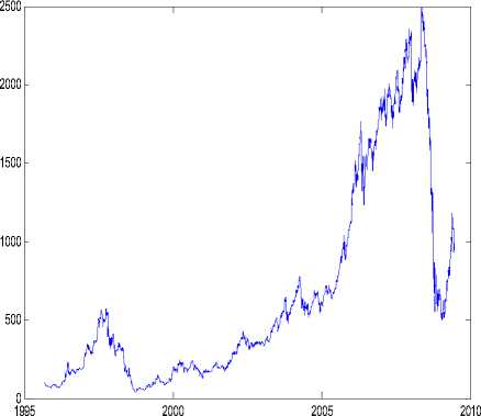
a) daily dynamics of index values

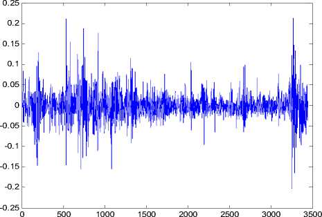
b) log daily losses

Fig. 1. RTSI Index – sample period 01.09.1995 – 30.06.2009 (closing values)

In addition to this, Jarqua-Bera statistic shows that law of log daily losses is obviously different from normal distribution. The JB test statistics is defined as [10]:

IR — П STD 2 i ( Kurtosis - 3) 2

JB 6 [ 6 +      24     ] •

The JB statistic has approximately a chi-squared distribution, with two degrees of freedom. The Jarqua-Bera test depends on skewness and kurtosis statistics. If the JB test statistic equals zero, it means that the distribution has zero skewness and kurtosis is about equal 3, and so it can be concluded that the normality assumption holds. Skewness values far from zero and kurtosis values far from 3 lead to an increase in JB values. The test returns the logical value h = 1 if it rejects the null hypothesis at the p <0.05 significance level, and h =0 if it cannot. We have for data of Table 1: JB value=6532.8 , p ~0, h =1. It means that we can reject the hypothesis that the distribution of daily losses is normal.

Table 1. Summary statistics for daily losses in RTS

mean	min	max
-0.0007	-0.2020	0.2120
std	skewness	kurtosis
0.0289	0.3752	9.7024
variance	JB test	n
-0.0008	6532.8 h=1,p <0.001	3447

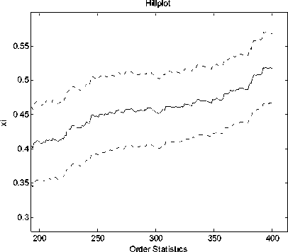
In Fig.2 we represent the Hill graph, which plots the Hill estimator of ξ , versus the k upper order statistics (and threshold u , respectively). We select the last area to k~0.1*3447~350, where the Hill estimator is more stable.

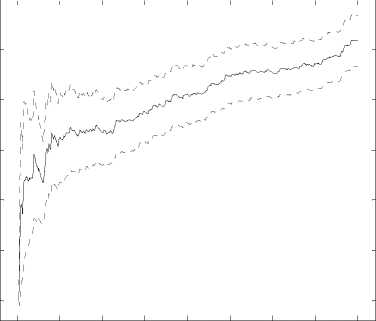
The mean excess function (7) allows to establish the behavior of the distribution tails [23]: we choose threshold u looking at the linear shape (with positive slope) of the graph (Fig.3). Considering Hill plot and the mean excess function, we choose u =0.0334 (the number of observation exceeding threshold u is equal k =294).

The results of ML estimation of the GPD parameters                                =0.1492

and β = 0.0206:

Maximum Likelihood (ML) estimates of ξ,β: out = par_ests: [0.1492 0.0206]

funval: -803.6979

par_ses: [0.0688 0.0018]

threshold: 0.0334

data: [1x294 double]

p_less_thresh: 0.9675

QQ-plot graph makes us able to evaluate the goodness of fit of the empirical series to a parametric GPD model (Fig.4) [24]. Notice that a concave departure from the straight line in the QQ-plot (Fig.4a) is an indication of heavy tailed distribution, whereas a convex departure is an indication of a thin tail.

After we get estimates ξ,β, use them in (5), get the formula for of tail evaluation:

k(u)           x - 0.0334 -— p = F(x) = 1--(1 + 0.1492*-----------) 4 2

n               0.0206

k ( u ) = 294, n=3447, k(u)/n=8.53%

Employ the result in (6), get the VaR formula on GPD model:

VaR, = 0.0334 + ^0.02⁰⁶{[3447(i - p )] ^{- 0}4492 - 1}. ^p           0.1492 294

In Table 2 we report 95%, 99%, 99.5%, 99,9% Value-at-Risk estimates of three different VaR estimation methods. The performance of the different VaR estimation methods can be evaluated by comparing the estimates with the actual losses observed, in particular by computing (and testing) the number of VaR violations. VaR approaches based on the assumption of normal distribution are – 116 –

Hillplot

0.5

0.4

0.3

0.2

0.1

0     50    100   150   200   250   300   350   400

Order Statistics

a) Hill estimator versus k upper order statistics (k≤350)

b) Hill estimator versus k upper order statistics (k≤350) (plot zooming)

Fig. 2. Hill estimator versus k upper order statistics (probability level p=0.95)

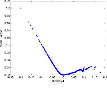
Fig. 3. Mean excess function

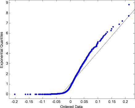
а) QQ-plot: empirical vs exponential distribution

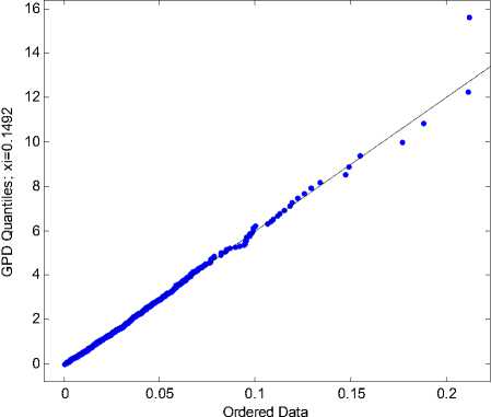
b) QQ-plot: empirical vs GPD distribution ( ξ=0.1492, β=0.0206, u=0.0334)

Fig. 4. QQ-plot versus GPD distribution and exponential distribution

Table 2. VaR estimation for daily RTSI losses:one day horizon

VaR approach p=0.950 p=0.975 p=0.990 p=0.995 p=0.999 Normal model 0.0394 0.0451 0.0520 0.0565 0.0663 Historical simulation 0.0452 0.0607 0.0849 0.1083 0.1771 GPD model 0.0499 0.0611 0.0856 0.1062 0.1620 definitely to underestimate high percentiles, while estimates based on historical simulation face with the problem of out of sample performance. The extreme value approach on GPD model seems appropriate and easy to implement.

Conclusions

Since last century, volatility of international financial system is getting severe. A stable financial system is so desirable. Therefore, risk management has aroused growing attention. As a measurement of market risk, VaR has been widely used in risk management. However, derivation between VaR estimation of normal hypothesis and abnormal distribution of practical benefit rate of financial always cause the bigger error in estimation. Aiming at this problem, through GPD model which fits tail distribution of financial products more accurately, this paper recalculates VaR by POT method. Compared with traditional method of risk study, this paper has made some progress in research approach and philosophy and more applicable in practice, which has been demonstrated by example of the Russian market analysis.

We use software systems: EVIM [25,26], MATLAB [27] and LOGOS-EVT, developed by authors of this paper.

Россия, Железногорск, ул. Кирова, 12а в ТелекомСтройСервис Россия 302528, Орловская обл., п. Зареченский, ул. Царев Брод, 61

При моделировании поведения фондового рынка обычно используется нормальное распределение Гаусса. Однако, метод превышений порога (РОТ) теории экстремальных значений (EVT), обобщенное распределение Парето (GPD) позволяют более точно описывать финансовые доходности (потери) от операций с ценными бумагами, особенно на хвостах вероятностных распределений. В данной работе описывается применение предложенных методов к моделированию и анализу потерь на основе индекса РТС, представляющего собой усредненную цену акций 50 крупнейших российских компаний, за 15-летний период (1995 - 2009 г.). Особое внимание уделено использованию предложенных методов для оценки экстремального рыночного риска на хвостах распределений, что позволяет получить современный инструмент моделирования для системы управления рисками.