Factorial Design-Based Optimization of Fuzzy Logic Controller Parameters for Autonomous Robot Navigation in Static Environments

Navigating autonomously in unknown environments remains a significant challenge for mobile robots, largely due

This work is open access and licensed under the Creative Commons CC BY 4.0 License.

to the unpredictable nature of sensor data, varying environmental conditions, and the nonlinear behavior of robot dynamics [1]. Successful navigation depends on the integration of several complex tasks such as perception, localization, path planning, and motion control which must work together seamlessly [2]. Among these, path planning is particularly difficult because of the inherent uncertainty and imprecision in sensor inputs [3]. As autonomous robots are increasingly deployed across a wide range of fields including logistics, security, agriculture, healthcare, and space missions their ability to navigate accurately and independently has become more critical [4].Fuzzy Logic Controllers (FLCs) have proven to be effective in addressing the inherent uncertainties of autonomous systems by leveraging linguistic variables and fuzzy membership functions (MFs). In contrast to traditional control strategies that depend on precise mathematical modeling, FLCs mimic aspects of human reasoning, enabling more flexible and adaptive behavior in the face of dynamic and ambiguous inputs [5]. As a result, their use in autonomous robotics has grown considerably, with numerous studies highlighting their strong performance in complex and unpredictable operating environments as reported [6]. Despite their advantages, performance of Fuzzy Logic Controllers (FLCs) is highly dependent on key design choices, particularly the size of the rule base, type of membership functions used, and approach to sensor fusion. A poorly constructed rule set can introduce unnecessary computational complexity, while an ill-suited membership function may hinder the controller’s ability to respond in real time. Likewise, if sensor fusion is not carefully optimized, it can produce noisy or delayed signals, ultimately compromising the robot’s navigational accuracy and efficiency [7]. Although previous studies have explored these factors independently, a systematic evaluation of their combined influence remains limited in static unknown environments. Addressing this research gap, the study employs a 3×3×3 factorial design to systematically evaluate the interactions between fuzzy rule sets, sensor fusion levels, and membership functions. Utilizing a co-simulation framework combining MATLAB fuzzy logic control and CoppeliaSim robot simulation, the study aims to identify optimal configurations enhancing navigation efficiency and robustness. Each scenario undergoes statistical analysis through threeway ANOVA analysing traversal time data collected over three replicates per configuration totalling to 81 simulation runs. This research provides a significant contribution to fuzzy logic controller design, proposing a framework for optimizing robot navigation parameters, with practical implications for embedded and real time robotic systems.

Research Hypothesis

Based on the conceptual frame work and objectives of this research work, the following hypotheses direct the conduct and analysis of this research.

H₀ : Null Hypothesis

H 1 : Alternative Hypothesis

Let

A i represents fuzzy rules’ effect

B j represents sensor fusion’ effect

C k represents membership function’ effect

AB (ij) represents fuzzy rules and sensor fusion interaction’s effect

AC (ik) represents fuzzy rules and membership function interaction’s effect

BC (jk) represents sensor fusion and membership function interaction’s effect

ABC (ijk) represents fuzzy rules, sensor fusion and membership function interaction’s effect.

H₀: A_l = 0 “There is no significant difference in the number of fuzzy rules’ effect on navigational time of nonholonomic wheeled path planning robot in unknown static environment”

H 1 : A_l ^ 0 “There is significant difference in the number of fuzzy rules’ effect on navigational time of nonholonomic wheeled path planning robot in unknown static environment”

H₀ : B j = 0 “There is no significant difference on sensor fusion’ effect on navigational time of nonholonomic wheeled path planning robot in unknown static environment”

H 1 : B j ^ 0 “There is significant difference on sensor fusion’ effect on navigational time of nonholonomic wheeled path planning robot in unknown static environment”

H₀ : C_k = 0 “There is no significant difference on membership functions’ effect on navigational time of nonholonomic wheeled path planning robot in unknown static environment”

H 1 : C_k ^ 0 “There is significant difference on membership function’ effect on navigational time of nonholonomic wheeled path planning robot in unknown static environment”

H₀ : AB ij = 0 “There is no significant difference on fuzzy rules and sensor fusion’ effect on navigational time of nonholonomic wheeled path planning robot in unknown static environment”

H 1 : AB_l j Ф 0 “There is significant difference on fuzzy rules and sensor fusion’ effect on navigational time of nonholonomic wheeled path planning robot in unknown static environment”

H₀ : AC_lk = 0 “There is no significant difference on fuzzy rules and membership functions’ effect on navigational time of nonholonomic wheeled path planning robot in unknown static environment”

H 1 : AC_lk Ф 0 “There is significant difference on fuzzy rules and membership functions’ effect on navigational time of nonholonomic wheeled path planning robot in unknown static environment”

H0 : BCjk = 0 “There is no significant difference on sensor fusion and membership functions’ effect on navigational time of nonholonomic wheeled path planning robot in unknown static environment”

H 1 : BC j _k &  0 “There is significant difference on sensor fusion and membership functions’ effect on navigational time of nonholonomic wheeled path planning robot in unknown static environment”

H₀ : ABC_l j _k = 0 “There is no significant difference on fuzzy rules, sensor fusion and membership functions’ effect on navigational time of nonholonomic wheeled path planning robot in unknown static environment”

H 1 : ABC_l j _k ^ 0 “There is significant difference on fuzzy rules, sensor fusion and membership functions’ effect on navigational time of nonholonomic wheeled path planning robot in unknown static environment”

Partitioning the sum of square for three factor factorial design with ‘n’ replicates per cell. The model is defined as equation.1.

= 1,2,... ,aAt a levels of factor A = 1,2,... ,b At b levels of factor B = 1,2,... ,c At c levels of factor C = 1,2, ,.,n At n replicates per cell

^yl;kl = В + ^A l + ^B j + ^C k + ^(AB) ; + ^(AC) lk + (BQ jk + ^{(AB C)} jk + ^e l;kl ^{ ^

where, y_l j _kl is a response in 1’th replicate with factors A, B, C at levels i, j, k, respectively; ц is the base line mean effect; A_l,B j and C_k , are main effects of factors A,B, C at levels i, j, k, respectively; (AB')_l j is the effect of the interaction between A_l and B j , (AC)_lk is the effect of the interaction between A_l and C_k ; (BC) j _k is the effect of the interaction between B j and C_k, ; (ABC)_l j _k is the effect of the three-factor interaction between A_l, B j and C_k , and and finally e_l j _kl is a random error of the kth observation from the (I,j,k)th treatment.

2.    Related Works

Fuzzy Logic Controllers (FLCs) have gained substantial attention in the field of mobile robot navigation, largely due to their ability to handle uncertainty and adapt effectively to complex environments. Early works in this area were primarily concerned with establishing the fundamental feasibility of fuzzy control systems for navigation tasks [8-9]. More recent research has shifted toward refining these systems, focusing on techniques such as optimizing membership functions, streamlining rule bases, and improving sensor fusion methods to enhance overall performance.

Štefek et al. (2021)[10] investigated the use of genetic algorithms to optimize membership functions, reporting notable improvements in controller responsiveness during navigation. In a related vein, Seines and Babuška (2001)[11] examined methods for reducing the size of fuzzy rule bases, demonstrating that a more compact set of rules can substantially lower computational demands without compromising navigational accuracy. However, both studies primarily addressed these design parameters independently, offering limited insight into how these factors might interact when tuned simultaneously.

Sensor fusion remains a cornerstone of robotic perception, drawing considerable interest for its role in enhancing environmental awareness and mitigating uncertainty. Almasri (2016)[13] demonstrated that integrating multiple sensor significantly improves perception accuracy and leads to more reliable obstacle avoidance. More recently, Abbasi et al. (2023) [14] emphasized the benefits of adopting moderate levels of sensor fusion, noting that a balanced approach can enhance navigational performance while avoiding excessive computational overhead.

While recent research has advanced several dimensions of FLC optimization, many studies still fall short in examining the combined effects of key parameters. For example, Wang (2022) [16] employed adaptive fuzzy control techniques in dynamic environments and reported gains in obstacle avoidance, yet did not investigate how sensor fusion interacts with membership function design. Similarly, Khudaverdiyeva (2022)[17] showed that optimized rule sets can enhance navigational efficiency but did not account for the influence of sensor fusion levels. In related work, Pham et al. (2023) [18] and Muralidharan, Romero and Wuthrich (2021) [19] focused on refining membership functions to support energy efficient navigation but overlooked the interplay between rule base size and sensor integration strategies. In this study [20] real-time fuzzy logic control using multiple sensor inputs was explored; however, their work did not include a systematic analysis of how different sensor fusion levels interact with rule base reduction or membership function variation. Similarly, Herrera Ortiz et al. (2013)[21] applied evolutionary algorithms to optimize fuzzy controllers but did not investigate the role of sensor fusion in their optimization framework. Silva, Rabelo and Santana (2014) [22] addressed the effects of sensor noise on fuzzy controller performance, yet their study did not consider the combined impact of rule set size and membership function design. Patel et al. (2023) [23] focused on developing efficient rule based controllers but, like the others, examined design parameters in isolation, without addressing their interdependencies.

The present study addresses this critical gap by employing a factorial experimental design to systematically evaluate the interaction effects among key fuzzy controller parameters. Through statistical analysis, this research identifies optimal configurations for fuzzy logic controllers, offering both theoretical insights and practical guidelines for enhancing autonomous navigation in static, unstructured environments.

3.    Proposed Approach

This section presents the experimental framework developed to assess how three critical parameters of fuzzy logic controllers (FLCs), rule base size, sensor fusion level, and membership function (MF) type influence the navigational performance of a nonholonomic wheeled mobile robot. A factorial experimental design was employed within an integrated simulation environment, supported by statistical analysis, to ensure methodological rigor and facilitate reproducibility of the findings.

• 3.1.    System Architecture and Experimental Framework

• 3.2.    Fuzzy Logic Controller Design

The architecture consists of three core components CoppeliaSim Environment, MATLAB Controller Engine and Communication Interface (Remote API).

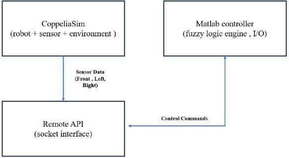
Fig.1. System architecture- MATLAB CoppeliaSim co-simulation

The fig.1 describes the integration architecture between MATLAB and CoppeliaSim using a Remote API. CoppeliaSim acts as the simulation environment that contains the robot, sensors, and the simulated environment. It generates and sends sensor data to the Remote API. MATLAB serves as the computational engine for the FLC, managing sensor data processing, fuzzy inference logic execution, and control command generation. CoppeliaSim, on the other hand, provides a realistic and interactive 3D simulation environment modelling the physical properties and kinematics of a nonholonomic wheeled robot platform. The simulation environment is designed as a static, maze-like obstacle course measuring 5 m × 5 m square, populated with fixed cylindrical obstacles to emulate challenging navigation conditions.

Sensor data from ultrasonic sensors mounted on the robot chassis, are continuously collected by CoppeliaSim and transmitted to MATLAB through the Remote API. MATLAB processed this data through the FLC and computes corresponding wheel velocity commands. These commands were then sent back to CoppeliaSim to control the robot's movements in real-time, thus closing the control loop.

The experimental framework employed a factorial design involving three primary variables: rule set size (27, 18, and 14 rules), sensor fusion levels (minimal, moderate, and dense), and membership function types (triangular, trapezoidal, Gaussian). The main performance metric captured was the traversal time which provide quantitative insights into the effectiveness and efficiency of each tested fuzzy logic configuration. While traversal time serves as a primary quantitative indicator of navigational efficiency, it represents only one dimension of performance. Future evaluations should incorporate additional metrics such as path smoothness, obstacle clearance, control stability, and energy efficiency to provide a more holistic assessment of robot behavior.

Ultrasonic sensor circuit was used to measure the crisp distance value between the robot and obstacles. The sensor data provided information regarding obstacles presence in the trajectory. If the robot was near an obstacle, it adjusted its speed respectively.

As in fig.2, inference engine was partitioned into four segments. The fuzzifier handles the task of gauging input variables, conducting scale mapping, and carrying out fuzzification. It entails the conversion of calculated signals (crisp values) into fuzzy values, which are also referred to as “linguistic variables”. Membership functions (MFs) were utilized for this transformation. The membership function, ranging from 0 to 1, represents the extent to which something belongs to a particular fuzzy set. If it is certain that the quantity belongs to the fuzzy set, its value is 1; conversely, if it is certain that it does not belong to the set, its value is 0.

The controller receives three directional distance inputs derived from sensor fusion strategies Left Distance (dl), Front Distance (df) and Right Distance (dr) obstacle proximity on the robot respectively. Each input is normalized to a range [0, 1] and described using three linguistic terms Near: Object is close and requires evasive action, Medium: Moderate distance may require steering adjustment and Far: Clear path in the sensed direction.

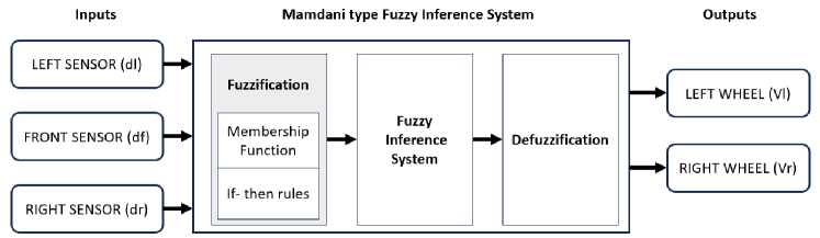
Fig.2. The fuzzy logic models [24]

• 3.3.    Membership Functions (MFs)

Membership functions defined how input values were assigned degrees of membership within fuzzy sets. Three MF types were used in experimentation ie triangular, trapezoidal and gaussian MF.

Triangular MF define by 3 parameters (a,b,c) is fastest to compute and widely used in real time systems, defined by equation 2.

x—a b—a c—x c—b if x < if a < x if b < x if x>

Trapezoidal MF, defined by four paramenters (a,b,c,d) and provides plateau for stability in output using equation 3.

ц trapezoid = max

(min ( — ,1,^,0) b—a   d—c/

The typical representation of the Gaussian membership function is Gaussian(x:c,s), where c, s stands for the mean and standard deviation. Here, c stands for the center, s for the breadth, and m for the fuzzification factor as in equation 4.

ц_л(х,с,5,т) = exp |- 1 1^1 |

The selection of triangular, trapezoidal, and Gaussian membership functions was guided by their prevalence in fuzzy logic control literature and their contrasting computational characteristics. These three represent a balanced spectrum, triangular functions provide sharp linear transitions and require only three parameters, making them computationally efficient for real time applications; trapezoidal functions introduce a plateau that improves stability at the cost of one additional parameter; and Gaussian functions offer smooth, differentiable curves that better handle noisy inputs but demand greater computational effort. Other families such as bell-shaped or sigmoidal functions were not included to maintain experimental tractability and focus on commonly adopted MF shapes.

• 3.4.    Rule Base

The FLC uses a knowledge driven rule base that encodes expert control strategies using IF–THEN linguistic rules. The rules determine how input conditions map to velocity commands examples are shown below.

Rule l: If dl is S and df is S and dr is S, then V L is L and V R is L.

Rule 2: If dl is S and df is S and dr is M, then V L is M and V R is L……….

The rule base reduction followed a structured expert pruning approach. Starting from the full 27-rule combination, redundant or overlapping rules were identified by analyzing similar antecedent and consequent relationships. These were consolidated based on symmetry and similarity in obstacle avoidance behavior, producing the 18-rule set. A further expert review eliminated low impact rules whose activation strength remained minimal across simulations, resulting in a 14-rule minimal configuration. This hybrid pruning process balanced interpretability and coverage, ensuring that all essential navigational behaviors e.g., obstacle avoidance and path correction remained intact while minimizing computational overhead. Reducing the number of fuzzy rules has direct computational and memory advantages that are crucial for deployment on embedded microcontrollers. Each rule introduces multiple antecedent evaluations, fuzzy set look-ups, and consequent activations that must be stored and executed in real time. A smaller rule base therefore reduces both inference latency and RAM usage, enabling faster control cycles and lower energy consumption. For instance, the 14-rule configuration executes roughly half the number of logical evaluations required by the 27-rule set, resulting in a noticeably lighter processing load during co-simulation.

The FLC outputs two control signals, the left wheel velocity (V L ) and right wheel velocity (V R ) each output used three linguistic terms: Low, Medium and High. These outputs were also defined using triangular membership functions. After rule evaluation, the controller aggregates all output fuzzy sets and converts them into crisp values using centroid defuzzification equation 5. This approach facilitated a seamless and interpretable conversion of fuzzy logic outputs into executable motor commands.

output =

J х^ ^ (х~)(1х

J РлЮах

To assess the performance of various fuzzy logic controller configurations under controlled yet realistic conditions, a detailed simulation environment was developed using CoppeliaSim. This environment closely emulated real-world navigation scenarios encountered by nonholonomic wheeled mobile robots operating in static, unknown environments. It offered precise modeling of the robot’s kinematics, dynamics, and sensor feedback, making it well-suited for the development and evaluation of autonomous navigation algorithms.

• 3.5.    Mobile Robot Model

Pioneer 3-DX is a widely adopted robotic platform known for its versatility and support for a broad range of sensors and interfaces, making it particularly well-suited for both research and educational purposes. Its adaptability, and seamless integration with various programming environments, including the Robot Operating System (ROS), have made it a valuable asset in robotics development and experimentation [25].

The robot model utilized in this study follows a unicycle-type mobile robot configuration. It employs two independently driven wheels, allowing for precise control over both linear movement and rotational orientation [26]. Fig.3 illustrates the robot model and sensor arrangement; it is equipped with eight ultrasonic proximity sensors distributed across its front. The sensors are positioned at angles ranging from –90° to +90°, with identifiers from 0 to 7. These sensors provide distance readings for detecting obstacles, which serve as inputs to the fuzzy logic controller.

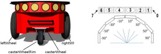
Fig.3. Pioneer P3dx. Robot model and sensor arrangement

Our experimental model was informed by and builds upon the methodologies and insights presented in prior research, including the works [27-28-25]. Fig.4 illustrate the kinematic and dynamic model of a two-wheeled mobile robot with a non-holonomic differential drive system. The term non-holonomic describe the “robot's failure to execute sideways motions and its dependence on the rolling-wheel concept”.

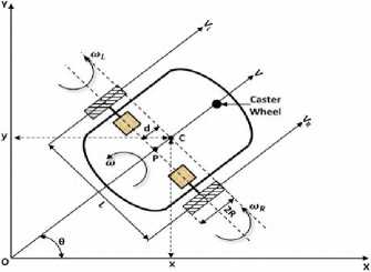
Fig.4. Kinematic and dynamic model [29]

In the Kinematic and dynamic model L, R, and C denotes the track width, radius of the wheels, and center of the mass of a mobile robot, respectively. The point P is located between the centers of the driving wheels axis. The point d is the distance between the points P and C. The landmark (O, X, Y) shows the field navigation environment, and (O, x, y) is the moving axis of the mobile robot. The θ is the turning angle, which represents the orientation of the robot about an axis (O, X). The three parameters (x, y, θ) describe the initial posture of the mobile robot.

The linear and angular velocities of the robot can be expressed in terms of the wheel velocities as in equations 6 and 7:

.

L у _ Vr+Vi

The Final Discrete-Time Update Equations developed from equations 6 and 7 are 8,9 and 10 for robot motion.

xt + 1 = xt + Vv+V . cos (d^.At(8)

к + 1 = к + ^^sin (O; Ml

6t + 1 = 6t+^.At(10)

These equations were used at each simulation time step to compute the next pose (x,y,θ) of the robot based on FLC outputs Vl and Vr. FLC uses distance sensors dl,df,dr to infer Vl and Vr, the above kinematic model then propagates the robot's pose for each step to form a closed-loop control system . At each time step we get sensor input from left right and front sensors then Fuzzy controller determines Vr and Vl. using Discrete-Time Update equations.

Additional details regarding its application is in the analysis by Nurmaini & Chusniah (2017) [30] . which offers solution for conducting this experimental simulation. In this context, V_r and V i represent the linear velocities of the right and left wheels, serving as the motion commands for navigating the mobile robot.

In the path planning procedure, the robot needed to coordinate obstacle detection with path planning. The expectation was that obstacle avoidance would be achieved when robot reacts efficiently and devises a path free of collisions using sensor data from its environment. In this study, a fuzzy controller mimicking human driving intelligence was used.

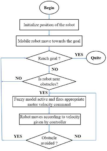
Fig.5. Navigational flowchart

The navigational flowchart in fig.5 illustrates the control logic for navigation. The process begins with initializing the robot’s position, and the robot then attempts to move toward the goal. If the goal is reached, the process ends. If not, the robot checks its sensors to determine whether it is near an obstacle. If no obstacle is detected, it continues moving toward the target. If an obstacle is detected, the fuzzy logic controller is activated to provide the appropriate motor velocity commands. The robot then adjusts its movement according to these commands until the obstacle is avoided, at which point it resumes moving toward the goal. This cycle of sensing, decision-making, and control continues until the robot successfully reaches its destination.

• 3.6.    Unknown Environment Design

The simulation field shown in fig.6 was designed as a square enclosure measuring 5 meters in length and 5meters in width to confine the robot and ensure a consistent testing environment. The “unknown environment” in this study refers to a static maze-like layout with fixed, non-overlapping cylindrical obstacles distributed throughout the field. The arrangement was designed to combine wide open zones, narrow corridors, and dead-end passages, requiring the robot to execute multiple turns and obstacle-avoidance manoeuvres before reaching the goal region. Although the geometry of the arena remained constant during each trial, it was unknown to the controller. The robot possessed no pre-mapped path or global knowledge of obstacle locations. Navigation therefore depended entirely on reactive sensing through ultrasonic inputs and real-time fuzzy inference. This setup mimic practical indoor environments such as hallways or warehouse aisles where obstacles are stationary but spatial layout is not pre-programmed. It provides a reproducible yet sufficiently complex benchmark for evaluating path-planning intelligence under uncertainty.

The boundary ensured that the robot remains within the designated space. The inner maze featured walls with a thickness of 5 cm, a passage width of 30-50 cm to provide adequate room for navigation while maintaining a challenge, and a wall height of 20 cm to ensure obstacles are detectable by the robot's sensors. The field included twelve cylindrical obstacles, each with a diameter of 10 cm and a height of 15 cm. These obstacles were designed to simulate realistic scenarios for standard navigation tests and to be easily detectable by the robot’s sensors. The cylindrical obstacles were scattered throughout the field to test the robot's obstacle avoidance capabilities. The robot was positioned at the bottom left corner of the field, which served as the designated starting point for the simulation, challenging its navigation algorithm to maneuver efficiently in the constrained environment. The navigational environment is shown in Figure 6.

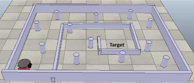
Fig.6. Navigational environment

The fuzzy logic controller parameters tested were Rule Set size at 14, 18, and 27 rules,Membership Function type including triangular, trapezoidal, and Gaussian, and Sensor Fusion level, tested at minimal, moderate, and dense fusion. The terminology corresponds to specific quantitative configurations in practice. “Minimal fusion” (Level 1) combines a limited subset of directional sensors (d0, d3, d4, d7) to represent left, front, and right zones. “Moderate fusion” (Level 2) averages grouped adjacent sensors (d0–d1, d3–d4, d6–d7) to provide balanced spatial perception. “Dense fusion” (Level 3) integrates all eight sensors (d0–d7) through full averaging as shown in figure 3. The choice of these levels was guided by the need to explore the trade-off between information richness and processing latency.

The fuzzy logic controller was implemented in MATLAB, and control signals are exchanged with CoppeliaSim via the Remote API. This setup allowed reading of real-time sensor data from the virtual robot, Execution of the fuzzy inference system in MATLAB, Real-time control of robot wheel velocities (V L and V R ) and Logging of simulation metrics. Each robot configuration was simulated for a maximum duration of 300 seconds. It should be noted that all experiments were conducted exclusively within a MATLAB-CoppeliaSim co-simulation environment under static, unknown obstacle configurations. The setting provides a controlled and repeatable testing framework; however, it lacks the unpredictability of dynamic obstacles and real-world sensor noise. Simulation platform was CoppeliaSim 4.4 with MATLAB 2022b integration. Hardware of Intel Core i7, 2.4 GHz, 16 GB RAM, 512 GB SSD and operating system: Windows 10 Pro (64-bit). A full factorial design was used to test 27 unique configurations of the fuzzy logic controller. Each configuration was subjected to three independent replicates, resulting in a total of 81 simulation runs.

• 3.7.    Data collection and Analysis

Data was collected primarily via experimental observation method. Collected data was analyzed using a factorial design analysis which involves partitioning the design model into appropriate Sum of Squares (SS) with respective degree of freedoms. The F tests on main effects and interactions follow directly from the expected mean squares in equation 11.

SS_T = та^ТЬ^Т^Т^у^ -

abcn

SST = Еа=1Е?=1Е£=1Е?=1У1%< — abcn

The sums of squares for the main effects are found from the totals for factors A(yi^,B(yj^ and C(y_k„) as in equations 12, 13 and 14.

SSa - -^У^У? - л   bcn L-1 L-

у.² .

abcn

'B =—'%-! У? - —

^D     acn ^{j 1 j} ' ^- abcn

- —y a 2 - ^y-

^C    abn^k- ¹^^- abcn

To compute the two-factor interaction sums of squares, the totals for the A x B, A x C, and B x C cells are needed. The sum of squares is found from equations 15, 16 and 17.

ssAB -jnya-iyM -a-n-ss*- ss*(15)

— SSsubtotal(AB) - SSA - SSB ssac = bn^a-^ytk -±n~ssA- SSc(16)

— SSsubtotal(AB)  SSA - SSB ss*c - antf-^y*       <^ SSc(17)

SSsubtotal(BC)   SSB

The three-factor interaction sum of squares is computed using equation 18.

SS abc -^ТТуЪ-^- SS a - SS b - SS c - SS ab - SS ac - SS bc

- SS_SU btotai(ABC) - SS a - SS b - SS c - SS ab - SS ac - SS bc

The error sum of squares is found by subtracting the sum of squares for each main effect and interaction from the total sum of squares as in equation 19.

SS_e - SS_t - SS_su btotal(ABC)                                      (19)

Collected data was analyzed using a factorial design approach, partitioning the model into Sum of Squares with respective degrees of freedom, as outlined in Table 1. Factorial design, an experimental design component, allows to investigate how multiple independent variables impact a dependent variable

Table 1. ANOVA for three-factor factorial design

Source of variation	Sum of squares	Degree of freedom	Mean square	F-ratio
A	SS a	(a-1)	SS a (a-1)	MS a mse
B	SS b	(b-1)	SS b (b-1)	MS b mse
C	SS c	(c-1)	ssc (c-1)	MS c mse
AB	SSab	(a-1)(b-1)	SSab (a-1)(b-1)	MS aAB MS~ e
AC	SSac	(a-1)(c-1)	SSac (a-1)(c-1)	MS ac mse
BC	SSbc	(b-1)(c-1)	SSbc (b-1)(c-1)	MS bc mse
ABC	SSabc	(a-1)(b-1)(c-1)	SSabc (a-1)(b-1)(c-1)	MS aABC mse
Error	SSerror	abc(n - 1)	SSerror abc(n - 1)
Total	SStotal	N-1

4.    Experiments

In this section, we present and analyze the outcomes of our 3×3×3 full factorial experiment, which evaluated the individual and combined effects of fuzzy rule base size, sensor fusion level, and membership function type on the navigation performance of a nonholonomic wheeled mobile robot within a simulated, static, unknown environment. A total of 81 trials (27 unique parameter combinations, each replicated three times) were conducted using the co‐simulation framework results described in table 1.

Table 2. 33 Factorial results of traversal time with 3replicates per cell

	27 fuzzy rules			18 fuzzy rules			14 fuzzy rules
	Trai MF	Trap MF	Gaus MF	Trai MF	Trap MF	Gaus MF	Trai MF	Trap MF	Gaus MF
Sensor fusion Level 1	176.16	180.15	180.39	176.29	178.96	179.58	170.58	176.47	176.14
	174.95	180.53	181.71	174.69	179.95	178.52	171.71	176.34	175.62
	175.88	180.96	180.31	174.75	178.61	180.27	170.32	175.86	176.0
Sensor fusion Level 2	169.81	175.04	175.51	169.38	175.19	174.51	161.98	172.22	170.77
	169.06	175.87	175.3	169.91	175.39	174.9	162.01	171.45	172.24
	167.84	176.23	176.8	168.23	173.72	175.51	160.22	170.67	171.41
Sensor fusion Level 3	174.58	179.41	178.46	174.28	178.73	178.37	169.31	175.25	176.75
	175.00	180.22	178.7	174.32	179.66	178.85	170.7	174.47	175.41
	175.72	178.31	180.66	173.9	181.23	178.22	171.1	176.26	175.86

Table 3. Anova results

Source of variation	Sum of squares	Degree of freedom	Mean square	F-ratio
Rule Set	38.1685	2	19.0843	32.5253
MF Type	54.2527	2	27.1264	46.2315
Sensor Level	40.6105	2	20.3053	34.6062
Rule Set × MF_Type	1.7936	4	0.4484	0.7642
Rule Set × Sensor Level	2.3755	4	0.5939	1.0122
MF Type × Sensor Level	31.5334	4	7.8834	13.4356
Rule Set × MF Type × Sensor Level	15.2331	8	1.9041	3.2452
Error (Residual)	31.6845	54	0.5868	—
Total	215.6518	80	—	—

Findings from table 2. Shows Main effects including Rule Set, MF Type, and Sensor Level all have large F-values (>30), indicating statistically significant main effects on the response variable. The two-way interactions shows that MF Type and Sensor Level show a strong significant interaction (F = 13.4356), suggesting a non-additive effect when these two are combined. Rule Set × and MF Type and Rule Set and Sensor Level have low F-values (<1.1), suggesting no significant interaction between those pairs. Three-way interaction with Rule Set, MF Type × Sensor Level has a moderate F-ratio (3.2452), indicating a potentially significant complex interaction across all three factors. Residual/Error Contains unexplained variance. The relatively low MS Error = 0.5868 confirms that most variability is explained by the model. All main effects significantly influence traversal time. Two key interactions suggest that The benefit of increasing the rule set might vary depending on the sensor fusion strategy. Membership function types might not perform consistently across different rule sets.

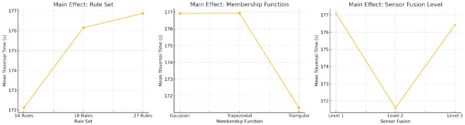
Fig.7. Main effects plot

The fig.7 show the main effects of three factors Rule Set, Membership Function, and Sensor Fusion Level on the dependent variable, Mean Traversal Time (s). Main effects describe how the mean of the response variable changes across the levels of each factor. Main Effect of Rule Set had Levels: 14 Rules, 18 Rules, 27 Rules. The observation is that As the number of rules increases, the mean traversal time increases. The increase in traversal time with more rules suggests that larger rule sets may introduce processing overhead or greater decision-making complexity, leading to slower system response. Statistically supported by the ANOVA result (F = 32.53, p < 0.001), indicating a significant main effect.

Main Effect of Membership Function Type with levels: Gaussian, Trapezoidal, Triangular. It was observed that Gaussian and Trapezoidal produce similarly high traversal times. Triangular yields a notably lower traversal time. The Triangular MF likely offers a simpler or faster decision boundary, leading to more efficient traversal. The sharp drop in traversal time for Triangular MF indicates a strong main effect, as confirmed by the ANOVA (F = 46.23, p < 0.001). Trapezoidal and Gaussian may involve smoother but more computationally intensive membership calculations.

Main Effect of Sensor Fusion Level with: Level 1, Level 2, Level 3 shows that Sensor Fusion Level 2 results in the fastest traversal, possibly indicating an optimal balance between data integration and processing speed. Levels 1 and 3 may introduce too little or too much data fusion, degrading performance. ANOVA confirms this with F = 34.61, p < 0.001, implying the choice of fusion level significantly affects performance.

The interaction effects in this analysis reveal how the influence of one factor on traversal time depends on the levels of other factors, indicating non-additive relationships. While the interactions between Rule Set and both Membership Function and Sensor Fusion Level show mild trends visually, they are not statistically significant, suggesting their combined effects on performance are largely independent. In contrast, the interaction between Membership Function and Sensor Fusion Level is both visually pronounced and statistically significant, showing that Triangular membership functions paired with Sensor Fusion Level 2 lead to substantially improved traversal times. Furthermore, the three-way interaction among Rule Set, Membership Function, and Sensor Fusion Level highlights that the optimal configuration particularly under Sensor Fusion Level 2 requires a joint tuning of all three factors, with the combination of fewer rules and triangular membership functions offering the best performance. Fig.8 illustrates the interaction effects among the three fuzzy logic controller parameters explained next.

Rule Set and Membership Function interaction

The lines are not parallel, especially between the Triangular and Gaussian MFs. Triangular MF shows a drop in traversal time at 14 rules, while Gaussian/Trapezoidal increase slightly or remain high. This Indicates a mild interaction, the effect of Rule Set depends on the MF type. Triangular MF interacts differently with the rule complexity benefiting from fewer rules, while others do not. However, this interaction was not statistically significant in ANOVA (F = 0.7642), suggesting this visual trend is not strong or reliable.

Rule Set and Sensor Fusion Level interaction

The traversal time drops sharply at 14 rules for Sensor Level 2, but less so for Levels 1 and 3. Lines are not parallel; there's a slight crossover at 18 and 27 rules. Suggests a small interaction: The impact of Rule_Set on traversal time varies with Sensor Fusion level. Especially for Sensor Level 2, performance improves drastically with simpler rule sets. Again, ANOVA showed this as non-significant (F = 1.0122), so while visually suggestive, it's not statistically robust.

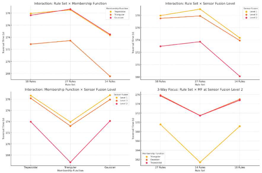
Fig.8. Interactions effects

Membership Function and Sensor Fusion Level interaction

Sensor Fusion Level 2 consistently results in lower traversal time across all MFs. The biggest dip occurs for Triangular MF and Level 2, with a clear non-parallel trend. Lines are well separated and show different slopes. This interaction is strong and statistically significant (F = 13.4356, p < 0.001). The effect of MF type depends heavily on the Sensor Fusion level. Triangular MF amplifies the performance benefit of Level 2 fusion and Gaussian/Trapezoidal behave more similarly across fusion levels. Indicates a non-additive synergy, where optimal MF and fusion levels must be jointly selected for best performance.

3-Way Interaction: Rule Set, MF and Sensor Fusion Level 2 interaction

Clear variation in performance across MFs and Rule Sets, only within Sensor Level 2. Triangular MF and 14 Rules results to lowest traversal time. Trapezoidal shows consistently worse performance, regardless of rule set. This is a subset view of the 3-way interaction. Suggests interaction effects are amplified under Sensor Level 2, Triangular MF and simpler Rule set optimal performance and Gaussian behaves moderately, Trapezoidal degrades consistently. ANOVA confirmed this 3-way interaction is statistically significant (F = 3.2452, p = 0.0044).

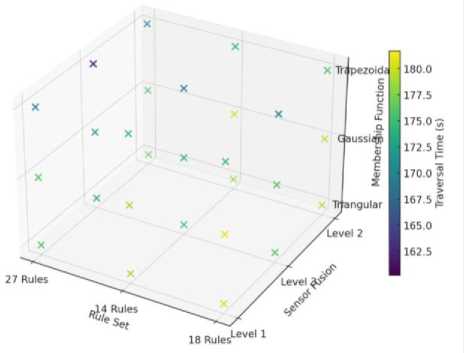
Fig.9. 3way interaction: traversal time over all factors

The 3D plot provided in fig.9 is a response surface visualization of the three-way interaction among Rule Set, Sensor Fusion Level, and Membership Function on the dependent variable Traversal Time (s) . This plot illustrates how traversal time is influenced by various combinations of these three factors. Each point corresponds to a unique combination of the three factors. Color gradient reveals how traversal time changes across combinations. It shows that the best and worst performances arise from specific factor interactions.

Table 4. Technical conclusions

Factor	Observation
Rule Set	Fewer rules (14) often yield faster traversal likely due to reduced complexity.
Sensor Fusion	Level 2 optimizes traversal time indicates a performance "sweet spot".
Membership Function	Triangular MF is consistently optimal across many conditions.
3-Way Interaction	System performance depends on joint tuning of all three factors — interactions are strong and nonlinear.

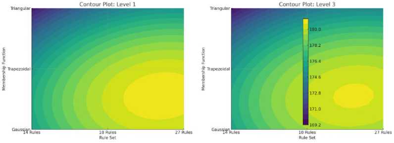
Fig.10. Contour plots

This response surface in fig.9 reinforces the importance of co-optimization in complex AI control systems: no factor operates in isolation. The best-performing configurations emerge from specific combinations , not from any single factor alone.

The contour plots shown in fig.10 presented provide a 2D visualization of traversal time across different combinations of two factors Rule Set (X-axis) and Membership Function (Y-axis) for two fixed levels of Sensor Fusion (Level 1 and Level 3). These plots help to understand how the response surface changes with these two factors at specific levels of the third factor.

Table 5. Summary of contour analysis

Aspect	Sensor Level 1	Sensor Level 3
Best Region	Triangular MF + 14 Rules	Still Triangular + 14 Rules, but Gaussian + 18 is closer
Worst Region	Gaussian MF + 27 Rules	Trapezoidal MF + 27 Rules
Response Shape	Smooth, concentric contours (simpler interaction)	Skewed, more complex contours (stronger interaction)
Implication	Independent optimization works	Joint optimization more critical

These plots visually confirm the interaction effect of Membership Function and Rule Set, and how this interaction changes across Sensor Fusion levels a hallmark of a 3-way interaction. Optimization strategies must therefore be context-aware, adjusting both fuzzy logic configuration and rule complexity in tandem with sensor integration design.

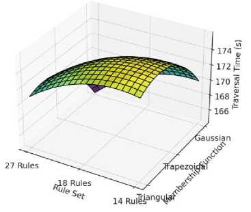
Fig.11. Response surface of sensor fusion level 2

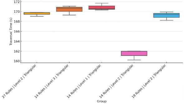
Fig.12. Traversal time comparison for top performing groups

The response surface in fig.11 for Sensor Fusion Level 2 shows how traversal time varies with rule set and membership function. The lowest traversal time occurs at the combination of 14 Rules and Triangular MF. Performance degrades i.e., traversal time increases with more complex rules or non-triangular membership functions. The surface shape confirms that main effects dominate, with minimal interaction curvature. This reinforces the statistical finding that Level 2, Triangular MF, and 14 Rules constitute the optimal fuzzy logic configuration. Although the 14-rule triangular-MF configuration with moderate (Level 2) sensor fusion yielded the fastest traversal times within the tested design space, this finding should be interpreted within its experimental bounds. The configuration represents a local optimum among the 27 factorially tested combinations rather than a globally optimal solution. Other untested configurations such as intermediate rule-base sizes (e.g., 16 rules), alternative membership function families, or different fusion algorithms could potentially yield superior performance under varying environmental conditions.

Moreover, this optimized configuration embodies a trade-off between computational efficiency, interpretability, and robustness. A smaller rule base and simpler triangular MFs accelerate inference and ease real-time implementation on embedded processors, yet may reduce behavioural richness and adaptability in more dynamic or noisy environments. Conversely, denser fusion or more complex membership functions can improve perceptual fidelity but impose heavier processing demands.

This boxplot in fig.12 compares the traversal time distributions for the top 5 best-performing combinations. It is evident that 14 Rules, Level 2 and Triangular has the lowest median and tight distribution, confirming it as the top performer. Other combinations have slightly higher times or wider spread, indicating less consistency.

Group

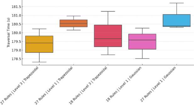
Fig.13. Traversal time comparison for worst performing groups

This boxplot in fig.13 displays the worst 5 performing combinations in terms of traversal time. These groups exhibit both higher medians and broader variability, reflecting slower and less consistent performance. Notably, combinations involving Trapezoidal or Gaussian membership functions at higher rule set and sensor fusion levels appear prominently.

Based on the surface plots and prior ANOVA results, we need an optimization strategy for minimizing Traversal Time using the interaction structure of Rule Set, Membership Function and Sensor Fusion Level. Objective is to Minimize Traversal Time (s) by selecting the optimal combination of the three factors.

Table 6. Optimal configurations identified

Sensor Fusion Level	Optimal Rule Set	Membership Function	Traversal Time Trend
Level 1	14 Rules	Triangular	Lowest traversal time (darkest region in contour)
Level 2	14 Rules	Triangular	Global minimum across all combinations.
Level 3	14 Rules	Triangular (or Gaussian)	Triangular remains best; Gaussian + 18 Rules acceptable

Optimization rules from observed patterns is to use simple rule sets (14 Rules). Lowering rule complexity consistently leads to faster traversal across all sensor fusion levels. Complexity (18/27 rules) introduces decision latency and increases response time. Sensor fusion level 2 is optimal as from contour and 3D plots indicate it offers the best tradeoff between data integration and processing load.

To provide a clearer view of performance differences, the average traversal times for the best and worst performing configurations were extracted from the 81 simulation runs. The best configuration 14 rules, triangular MF, and Level 2 (moderate) sensor fusion achieved an average traversal time of 162.0s (95 % CI), while the worst configuration 27 rules, trapezoidal MF, and Level 3 sensor fusion required 181.5s, representing a 10.8 % reduction in completion time under the optimized settings. The corresponding partial η² values from the ANOVA were approximately 0.42 for membershipfunction type, 0.37 for sensor-fusion level, and 0.33 for rule-set size, indicating that each factor explained a substantial portion of the variance in traversal time.

Rule set size strongly influenced performance because each additional rule increases both memory requirements and inference latency. Larger rule bases expand the decision space, but they also introduce overlapping and redundant antecedent conditions, which slow processing. The smaller 14 rule configuration, produced through expert driven rule pruning, reduced inference time while retaining essential navigational behaviours. This directly translates into reduced computational load a critical advantage for embedded microcontrollers with limited processing and memory capacity.

Membership function type also played a central role. Triangular MFs yielded the lowest traversal times due to their simple, piecewise-linear structure and three parameter definition, enabling faster fuzzification and defuzzification. Trapezoidal and Gaussian MFs, though smoother, required additional parameters and floating point operations, increasing computational overhead and causing delayed motor responses. The sharper boundaries of triangular MFs likely promoted quicker transitions between linguistic states, producing more decisive turning and speed adjustments during obstacle avoidance.

Sensor fusion level exhibited a non-linear relationship with performance. Moderate (Level 2) fusion achieved optimal results because it balanced perceptual completeness with computational efficiency. Minimal fusion (Level 1) provided insufficient spatial awareness, occasionally leading to late obstacle detection, while dense fusion (Level 3) introduced redundant and sometimes conflicting sensor data that increased processing time and induced minor steering oscillations.

Interaction effects further revealed how these factors jointly shape controller behaviour. The synergy between triangular MFs and Level 2 fusion indicates that crisp input partitioning works best when coupled with moderate, non-redundant perception. Similarly, the beneficial interaction between smaller rule sets and moderate fusion suggests that simplified reasoning complements balanced sensory abstraction, allowing the controller to make quick yet context-aware decisions.

Beyond statistical significance, these patterns have practical implications for real time robotic navigation. The identified configuration minimizes traversal time while maintaining computational feasibility, making it highly suitable for deployment on embedded processors such as ARM Cortex or Atmega architectures.

Overall, the findings demonstrate that the performance of fuzzy logic controllers cannot be improved by adjusting parameters in isolation. Instead, optimal navigation arises from co-optimization, balancing rule base complexity, membership function granularity, and sensor fusion density to achieve an efficient equilibrium between perception, reasoning, and control. This insight provides both theoretical and practical guidance for developing lightweight, high-performance FLCs for autonomous mobile robots in constrained environments.

5.    Conclusions