Fermion with three mass parameters in the uniform magnetic field

In the context of existence of the similar neutrinos of different masses, we examine a possibility within the theory of relativistic wave equations to describe particles with several mass parameters. In general, existence of more general wave equations than commonly used ones is well known within the Gel’fand-Yaglom formalism – see references [1-5].

In particular, models for a spin 1/2 particle with two and three mass parameters were developed [6–15]. Specific features of these models are as follows. For two (or three) bispinors, in absence of external fields separate Dirac-like equations are derived, they differ in masses. However, in presence of external electromagnetic field or gravitational field with non-vanishing Ricci scalar, the wave equation for bispinors does not split into separated equations, instead a quite definite mixing of two (or three) equations arises. It was shown that generalized equations for Majorana particle with several mass parameters exist as well. Such generalized Majorana equations are not trivial if the Ricci scalar does not vanish.

In the present paper, the model of a fermion with three mass parameters is studied in presence of the external uniform magnetics field. After applying the diagonalizing trans- formation, three separate equations are obtained effectively for particles with different anomalous magnetic moments. Their exact solutions and generalized energy spectra are found.

1. General theory in presence of electromagnetic and gravitational fields

We start with the system of equations for a fermion with 3 mass parameters [12, 15]:

iY ^a ( x )[ d a + Г a ( x ) + ieA a ( x )]Ф 1 ( x ) -

- M1 Ф1(x) + Y1S(x)Ф(x) = 0, iY a ( x )[ da +Г a ( x ) ieAa (x )]Фз( x) -

- M2Ф2(x) + Y2S(x)Ф(x) = 0, iY a ( x )[ da + Г a ( x ) + ieAa (x )]Фз( x) -

- M 3 Ф з ( x ) + Y 3 S( x )Ф( x ) = 0 , (1)

where the notations are used

^{Y 1} = ЗдЗ ^c 2 ^{( A} 1 ^{- c} 2 ) , i = ¹ , ² , ³ , L = ^c 1 ⁺ 3 , 3 M                         у о

Ф( x ) = L 1 Ф 1 ( x ) + L 2 Ф 2 ( x ) + L з Ф з ( x ) ,

Y₂L i = — ( A₂ - c ₂) x

• ²¹    3 M ^{( 2   2} )

• - L ( a ² + b ² ) + c 2 - c 2 ( A 2 + A 3 ) + A 2 A 3 ^{L ( A} 1 ^{- A} 2 ^{)( A} 1 ^{- A} 3 )

^Y 2 ^L 2 = 3 M ^{( A} 2 ^{- c} 2 ) ^x

• - L ( a ² + b ² ) + c 2 - c ₂ ( A 3 + A 1 ) + A 3 A 1 L ( A 2 - A 3 )( A 2 - A 1 )

^{Y 2 L 3} = 3 M ^{( A 2 - c 2} ) ^x

• - L ( a ² + b ² ) + c 2 - c ₂ ( A 1 + A 2 ) + A 1 A 2

^{L ( A} 3 ^{- A} 1 ^{)( A} 3 ^{- A} 2 )

^{Y 3 L 1} = 3 M ^{( A 3 - c 2} ) ^x

• - L ( a ² + b ² ) + c 2 - c 2 ( A 2 + A 3 ) + A 2 A 3

^{L ( A} 1 ^{- A} 2 ^{)( A} 1 ^{- A} 3 )

Y 3 L 2 = 3 M ^{( A} 3 ^- c 2 ) ^x

• - L ( a ² + b ² ) + c 2 - c 2 ( A 3 + A 1 ) + A 3 A 1

L ( A 2 - A 3 )( A 2 - A 1 )

S( x ) = -ieF ae ^ ^ae ( x ) + 4 R ( x ) ,

^-L|^c 4 | ^{2 -} Lc 3 | ^{2 + c} 2 ^{- c} 2 ⁽ A 2 ⁺ A 3 ) ⁺ A 2 A 3

^Lc 2 ^c 3 ^{( A} 1 ^{- A} 2 ^{)( A} 1 ^{- A} 3 )

^-L|c 4 1 ^{2 - L|c} 3 | ^{2 + c} 2 ^{- c} 2 ^{( A} 3 ^{+ A} 1 ) ^{+ A} 3 ^A 1 ^Lc 2 ^c 3 ^{( A} 2 ^{- A} 3 ^{)( A} 2 ^{- A} 1 )

• ^{- L|c} 4 | ^{2 - L|c} 3 | ^{2 + c} 2 ^{- c} 2 ^{( A} 1 ^{+ A} 2 ) ^{+ A} 1 ^A 2 ^Lc 2 ^c 3 ^{( A} 3 ^{- A} 1 ^{)( A} 3 ^{- A} 2 )

With the notation |c 4 | = a, |c ₃ | = b, the mixing matrix in the equation (1) is specified by the relations

^{Y 3 L 3} = 3 M ^{( A 3 - c 2} ) ^x

-L ( a ² + b ² ) + c 2 - c 2 ( A 1 + A 2 ) + A 1 A 2

^{L ( A} 3 ^{- A} 1 ^{)( A} 3 ^{- A} 2 )

We will consider eq. (1) in the cylindrical coordinates and tetrad     dS2 = dt2 - dr2 - r2dф2 - dz2, xa = (t,r,ф,z) ,

/1  0   00

в , л_ 10   1    0    0

e(a)(x)     [0   0   1 /r   0I

00  01

4 „

Y ¹ L ¹ = 3 M ^{( A 1 - c 2 ) x}

-L ( a ² + b ² ) + c 2 - c 2 ( A 2 + A 3 ) + A 2 A 3 ^{L ( A} 1 ^{- A} 2 ^{)( A} 1 ^{- A} 3 )

YL = ^-( A_x - c ₂) x

• ¹²    3 M ^{1   27}

  -L ( a ² + b ² ) + c 2 - c 2 ( A 3 + A 1 ) + A 3 A 1

L ( A 2 - A 3 )( A 2 - A 1 )

Y1L3 — —— ( A i — c ?) x

• ¹³    3 M^{v 1   27}

  -L ( a ² + b ² ) + c 2 - c 2 ( A 1 + A 2 ) + A 1 A 2 ^{L ( A} 3 ^{- A} 1 ^{)( A} 3 ^{- A} 2 )

Ricci rotation coefficients are as follows: Y ab 0 = 0 , Y ab 1 = 0 , y 122 = -Y 212 = 1 /r, Y ab 3 = 0 • The external magnetic field directed along the axis x ₃ is determined as follows

А ф = - 2 Br ² ,  F 12 ( x ) = F rф = -Br,

-ieF _ae ( x ) = -ieF ₁₂ ( x ) y 1 ( x ) y ² ( x ) = ieBY ¹ Y 2 =

= ieB

= eB S •

So, the main equation (1) takes the form (we simplify the notation, eB ^ B )

iY ^{0 d} + iY ^{1 d} + i² " (   + iBr " ) + iY ³ f! Ф 1

dt dr r \дф 2 / dz

-

-M Ф 1 + B S Y _L ( L 1 Ф 1 + L 2 Ф 2 + L 3 Ф 3 ) = 0 ,

'iY 0 d + iY 1 d + i^Y 2 ( d + B ) + iY 3 d l ^ф 2 at dr r \дф 2 ) dz

or

—M Ф 2 + B E Y ₂ ( L 1 Ф 1 + L ₂ Ф ₂ + L 3 Ф 3 ) = 0 ,

iY ^{0 d +} iY ¹ It ⁺ i^Y ∂t ∂r r

∂    Br ²

(дф ⁺ i 2)

∂

+ iY ³^- Ф 3 -

—M Ф 3 + B E Y 3 ( L 1 Ф 1 + L 2 Ф 2 + L 3 Ф 3 ) = 0 •

For three involved bispinors, we will use the following substitutions

ϵγ 0	+	iγ 1	∂ ∂r	γ 2 - rp ( r ) -	kγ 3	M
ϵγ 0	+	iγ 1	∂ ∂r	γ 2 - rp ( r ) -	kγ 3	M
ϵγ 0	+	iγ 1	∂ ∂r	γ 2 - rp ( r ) -	kγ 3	M

Ф 1 + p 1 EФ 1 = 0 ,

Ф₂+ p 2 EФ₂ = 0 ,

^Ф 3 ⁺ p 3 ^EФ 3 = ⁰ •

Ф 1 =      ■. Ф ⁱ ( f 1 ,f 2 ,f 3 ,f 4 )

Ф 2 =      ■ е^{г тф} е^{г к} ( g 1 ,g 2 ,g 3 ,g 4 ) t ,

Ф з = e- it^ e* ¹ _{( h} 1 ,h 2 ,h 3 ,h 4 ) t ,

Thus, after transformation, three separate equations are obtained effectively for particles with different anomalous magnetic moments.

2. Solving the basic equation

where () t stands for transpose. Then the previous system reads

£Y ⁰ + iY ¹ J-— — p ( r ) — kY ³ — M ∂r r

Ф 1 +

+( M — M 1 )Ф 1 + B E Y ₁ ( L 1 Ф 1 + L ₂ Ф ₂ + L ₃ Ф ₃ ) = 0 ,

£Y ⁰ + iY 1 о Y—p ( r ) — kY ³ — M ∂r r

Let us briefly describe the procedure for solving the basic equation (2):

₂                     Y f^л

£Y ⁰ + iY \— ст ( r ) — kY ³ — M + Г Z

∂r r f4

^{f 2} 1 = 0 • f ₃

Ф 2 +

+( M — M ₂ )Ф ₂ + B E Y > ( L 1 Ф 1 + L ₂ Ф ₂ + L ₃ Ф ₃ ) = 0 ,

Using the spinor basis for the Dirac matrices [3, 6], we obtain four equations

£Y ⁰ + iY ¹ Y—p ( r ) — kY ³ — M ∂r r

Ф 3 +

+( M — M 3 )Ф 3 + B E Y ; ( L 1 Ф 1 + L 2 Ф 2 + L 3 Ф 3 ) = 0 ,

—

i ( 4—+ ^p^) ^f 4 ^{+ ( £ + k} ) ^f 3 ^{+ (Г — M} ) ^f 1 = ⁰ , dr

—

i ( 4 p\ ^f 3 ^{+ ( £ — k} ) ^f 4 ^{— (Г + M} ) ^f 2 = ⁰ , dr

where

/1 0

/ \        , ¹_R 2 v I ^{0 — 1}

p ⁽ r ) = m ⁺ - Hr , ^E = 0 0

0 0

1 0

— 1

Using the shortening notations for elements of the mixing matrix

Zkj = (BYk) Lj = dk Lj, i ( 4—+ p^ f2 + (£ — k)f1 + (Г — M)f3 = 0, dr i ( 4p^) f 1 + (£ + k)f2 — (Г + M)f4 = 0 • (3) dr

Let dr ± p(r) = D±. Equations (3) can be considered as two linear subsystems and their solutions are we present the system as follows д Ф k + Zkj Ф j = 0,

f 1 = + i

( £ + k ) D + f 2 + (Г — M ) D + f 4

(Г — M ) ² — ( £ ² — k ² )    ’

d = E -

£Y ⁰ + iY 144"— — p ( r ) — kY ³ — M ∂r r

( £ — k ) D - f 1 — (Г + M ) D - f 3

⁺ i    (Г + M ) ² — ( £ ² — k ² )

The mixing matrix should be reduced to a diagonal form by a linear transformation

Ф = s Ф , д Ф = SZS - 1 Ф ,

µ1 0 0 SZS-1 = 0 µ2 0 0 0 µ3 f =_. (Г — M) D + f2 + (£ - k) D + f4 f3     i (Г — M )2 — (£2 — k2)     , f =_. ~(Г + M)D-f1 + (£ + k)D-f3

f ⁴ i (Г + M ) ² — ( £ ² — k ² )       •

Eliminating the variables f ₁ , f ₃ in the equations above, we obtain

As a result we get

	(ФЛ	µ 1		0	0	/ ФЛ
E - 1 d	Ф 2	+	0	µ 2	0	Ф 2	= 0 ,
	\ Ф3/		0	0	µ 3	\ Ф3/

Г + M £ - k ₌      D - D + f 2

Г — Mf ^{2 +} Г — Mf ⁴ (Г — M ) ² — ( £ ² — k ² ) ⁺

£ - k        D - D + f 4

⁺ Г — M (Г — M ) ² — ( £ ² — k ² ) , ⁽⁾

r + M ₌      D - D + f 2

€ + kf 4 (Г - M ) ² - ( € ² - k ² ) ⁺

Q ₁ = eB Un - 2 + Г ² - M ² -

Г - M      D - D + f 4

⁺ € + k ^X (Г - M ) ² - ( € ² - k ² ) ’

- k ² + € ² - 2Г V € ² - k ² •

Subtract the second equation from the first equation and substitute the resulting expression for f 2 into (4), so we obtain the fourth order equation for f 4 :

The variant II differs only in sign at the parameter Г . Thus, we are to solve two second-order differential equations:

d ⁴ f 4 + dr ⁴

e ² B ²

r ²

- eB (2 m - 1) -

- 2(Г ² - M ² - k ² + € 2 ) +

2 m ( m + 1) "| d ² f₄ dp" ⁺

r ²

+

_e 2 _B 2 _r

-

4 m ( m + 1)

df 4 + I e ⁴ B ⁴ dr 16

+ eB ^[ eB (2 m - 1) + 2(Г ² - M ² - k ² + € ² )] r ² -

_d 2     _B 2 _e 2 _r 2                ₁

dr 2-- — + eB mm - J ■ I - M 2 ^- k 2 +

+ , 2 + 2Г■ • k 2 -           ] f = 0 , (6)

_d 2     _B 2 _e 2 _r 2                ₁

dr 2-- — + eB m^- - ₂j+^r 2 - M 2 ^- k 2 +

+ € 2 - 2Г VS-k ? - m ⁽ m ₂ ⁺ *> ^] g = 0 •

-eB (2 m- 1)(Г2-M 2-k 2+€ 2) - (Г2 +M 2+k 2-€ 2)2 + e2B2

+4Г ² M ² 4—(6 m ² - 2 m - 1) +

m(m + 1)[eB(2m - 1) + 2(Г2 - M2 - k2 + €2)] +r- m(m - 2)(m + 3)(m + 1) , M

Г 4-------------- ^f 4 = ⁰ •      ⁽⁵⁾

Similarly, we can obtain the fourth order equation for the function f 2 . Equations for f 2 and f 4 turn out to be the same. To study the fourth order equation, we will use the factorization method:

F4 (r) f (r) = Л( r ) b2( r ) f (r) = 0, f2(r)= d + P0r2 + P1 + P2 , dr2

b2(r) =     + Q0r2 + Q1 + dr2

Computing the product

They differ only in sign at the parameter Г . Consider the equation (6). Let us make the change of the variable x = eBr ² / 2 . Solutions are constructed in the form f = x a e bx F . Taking into account the constraints a = -m/ 2 , ( m + 1) / 2 and b = - 1 / 2 , we obtain the equation for F :

xd-F + (1 + 2 a - x dx ²      2

dF dx

- 4 e 1 B [ eB (4 a + 1) - 4Г V€ ² - k ² - (2 m - 1) eB-

- 2(Г ² - M ² - k ² + € ²)j F = 0 •

It is an equation of the confluent hypergeometric type with parameters y=2 a+2,

d2

FI = I + P0r + P1 +--I X dr2

X (+ Q0r2 + Q1 + Д2^ dr2

and equating the result to the operator (5), we find two solutions for sets of numerical coefficients:

I   P ₀ = - 4 b ² e ² ,  p 2 = -m ( m + 1) ,

P ₁ = eB mm - I) + Г ² - M ² -

- k ² + € ² + 2Г V€ ² - k ² ,

II Q 0 = - 4 B ² e ² , Q 2 = - m ( m + 1) ,

a = - 4- B [ eB (4 a +1) - 4Г V€ ² - k ² - (2 m- 1) eB-

- 2(Г ² - M ² - k ² + € ² ) ] •

To construct solutions corresponding to bound states, one should use the positive values of the parameter a (for definiteness, we assume that eB >  0 ):

a = -m ( m< 0); a = m ±i >  0 ( m >  0) ^

The polynomial conditions а = -n ( let € ² - k ² = A ) provides us with the quantization rule for energy values

_ , 1 m , M2 - Г2 , Г VA ,   A a + 2 - "2 +  2eB + n = "bB + 2eB^

Hence, using the notation M ² + 2 eB ( a + 1 / 2 - m/ 2 + n ) = N, we obtain

A = ( ^VN - Г) ² >  0 •             (7)

ϵ

From (7) we find the formula for the energy values

- к^

M ² + 2 eB

1 — m A

—⁺ n)^— г

situation of an electrically neutral particle can also be carried out in the case of a particle with three mass parameters.

Depending on the value of a , we have two expressions for N :

3. Diagonalization of the mixing matrix

Let us turn back to the system of three equations

m< 0 , a = — —,

S

- 1

6Y ⁰ + iY 1т|— — И ( r ) — kY 3 — M ∂r r

Ф 1 +

б ² — к ² = [V M ² + 2 eB (1 / 2 — m + n ) — г] 2 ;

+( d 1 L 1 Ф 1 + d 1 L ₂ Ф ₂ + d 1 L ₃ Ф ₃ + ( M - M 1 )Ф 1 ) = 0 ,

m > 0,

m +1 a =   2 ’

S

- 1

6Y0 + iY 1т|—и (r) — kY3 — M ∂r r

Ф 2 +

б ² — к ² = [V M ² + 2 eB (1+ n ) — г] 2 .

+ ( d 2 L 1 Ф 1 + d 2 L 2 Ф 2 + d 2 L 3 Ф 3 + ( M — M 2 )Ф 2 ) = 0 ,

S

- 1

Thus, we obtain two series of energies

I :   X =( VN — Г) ² ; II : X =( VN + Г) ² .

6Y0 + iY 1т|—и (r) — kY 3 — M ∂r r

Ф 3 +

+ ( d 3 L 1 Ф 1 + d 3 L 2 Ф 2 + d 3 L 3 Ф 3 + ( M — M 3 )Ф з ) = 0 ,

Let us consider a special case of an electrically neutral particle with the magnetic moment (neutron). The transition

or briefly

to the case of a neutral particle can be carried out with the help of simple formal changes, e ^ 0 , X ^ ж, eX ^ Л ,

д = S -

6Y ⁰ + iY 17?— ~ И ( r ) — kY 3 — M ∂r r

so that

Г = Xe — ^ Г = ЛB. ℏ mc        mc2

д Ф k + T kj Ф j = 0 .

No additional calculations are needed. We obtain two second-order equations:

To find the transformation matrix S , which will diagonalize the mixing matrix, we are to study the following equation ST = T 0 S , or in detail

" d^ + (>6—2 + Г)2 — M 2 —      1 1 f = 0, dr2                                    r2

■£ +( V.   к _ Г) 2 — M 2 — mm ±P 1 f = 0 .

dr ²                                     r ²

General solutions of equations (8) have the form

s11   s12

s21   s22   s23I s31   s32

M

X

M 1 + d 1 L 1 d 2 L 1 d 3 L 1

d 1 L 2

M - M 2 + d 2 L 2

d 3 L 2

f ( r ) = V r ( J m +1 / 2 ( x ) + Y m +1 / 2 ( x )) , x = У ( V. ² — к ² + г) 2 — M ² r ;

g ⁽ r ) = Vr ⁽ J m +1 / 2 ⁽ У ) ⁺ Y m +1 / 2 ⁽ У )) , y = У ( V. ² — к ² — г )² — M ² r.

M

_

d ₁ L ₃

d ₂ L ₃

^M 3 ^{+ d} 3 ^L 3

µ 1

µ 2

⁰ I / ^s 11

0 I I s 21

µ 3      s 31

^s 12

^s 22

s ₃₂

^s 13

^s 23

s ₃₃

.

Hence we obtain three linear subsystems:

From the form of these equations, we can conclude that the magnetic moment manifests itself in an external magnetic field in a quite definite way: in fact, everything reduces to solutions with cylindrical symmetry for an ordinary free particle with spin 1/2, but with a certain replacement б2 — M2 ^ (V.2 — к2 ± г)2 — M2.

The main manifestation of the magnetic moment of a neutral particle is the modification (spatial scaling) of the wave functions in directions transverse to the magnetic field. Apparently, such a modification of the transverse structure of a neutron beam can be observed experimentally, for example, in neutron Bessel beams. Obviously, the transition to the

^{( M} — ^M 1 ^{+ d} 1 ^L 1 ) s 11 ^{+ d} 2 ^L 1 s 12 ^{+ d} 3 ^L 1 s 13 = ^и 1 s 11 , ^d 1 ^L 2 ^s 11 ^{+ ( M — M} 2 ^{+ d} 2 ^L 2 ) ^s 12 ^{+ d} 3 ^L 2 ^s 13 = И 1 ^s 12 , ^d 1 ^L 3 ^s 11 ^{+ d} 2 ^L 3 ^s 12 ^{+ ( M — M} 3 ^{+ d} 3 ^L 3 ) ^s 13 = И 1 ^s 13 ;

⁽ M — M 1 ⁺ d 1 L 1 ) s 11 ⁺ d 2 L 1 s 12 ^{+ d} 3 ^L 1 s 13 = ^и 1 s 11 , ^d 1 ^L 2 ^s 11 ^{+ ( M — M} 2 ^{+ d} 2 ^L 2 ) ^s 12 ^{+ d} 3 ^L 2 ^s 13 = И 1 ^s 12 , ^d 1 ^L 3 ^s 11 ^{+ d} 2 ^L 3 ^s 12 ^{+ ( M — M} 3 ^{+ d} 3 ^L 3 ) ^s 13 = И 1 ^s 13 ;

⁽ M — M 1 ⁺ d 1 L 1 ) s 31 ⁺ d 2 L 1 s 32 ^{+ d} 3 L 1 s 33 = И 3 ^s 31 , ^d 1 ^L 2 ^s 31 ^{+ ( M — M} 2 ^{+ d} 2 ^L 2 ) ^s 32 ^{+ d} 3 ^L 2 ^s 33 = И 3 ^s 32 , ^d 1 ^L 3 ^s 31 ^{+ d} 2 ^L 3 ^s 32 ^{+ ( M — M} 3 ^{+ d} 3 ^L 3 ) ^s 33 = И 3 ^s 33 .

Here we have three eigenvalue problems

M - M 1 + d 1 L 1 - ц 1		d 2 L 1 M - M 2 + d 2 L 2 - ц 1 d 2 L 3	d 3 L 1 d 3 L 2 M - M 3 + d 3 L 3 - ц 1/	s 11 s 12 s 13	= 0 ,
	d 1 L 2 d 1 L 3
M	- M 1 + d 1 L 1 - ц 2	d 2 L 1	d 3 L 1	s 21
	d 1 L 2	M - M 2 + d 2 L 2 - ц 2	d 3 L 2	s 22	= 0 ,
	d 1 L 3	d 2 L 3	M - M 3 + d 3 L 3 - ц 2/	s 23
M	- M 1 + d 1 L 1 - ц 3	d 2 L 1	d 3 L 1	s 31
	d 1 L 2	M - M 2 + d 2 L 2 - ц 3	d 3 L 2	s 32	= 0 .
	d 1 L 3	d 2 L 3	M - M 3 + d 3 L 3 - цг)	s 33

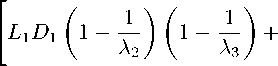
Note that the three rows of the matrix S may be found only up to arbitrary multipliers. The condition for the existence of solutions for these three systems is the vanishing of the determinant

/ M - M1 + d 1L1 - ц det          d1L2

d 1 L 3

d 2 L 1                   d 3 L 1

M - M2 + d 2 L 2 - ц        d 3 L 2         = 0.

d 2 L 3        M - M3 + d 3 L 3 - ц

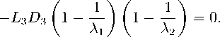
Let us get the explicit form of the third order equation for parameter µ:

+ M3 (1 -   (1 - ^V1 -

λ ₁          λ ₂          λ ₂

= 0 .

-ц 3 + (3 M-Mi-M2 - M3+d i L i+d 2 L 2+d 3 L 3) ц 2+ + [- d 1L 1(2M - M2 - M3) - d2L2(2M - M1 - M3) -

-d 3 L 3 (2 M-M2-M1) - 3 M 2+2( M1 + M2+M3) M -

- (M1 M2 + M1 M3 + M2 M3)] ц+

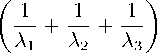
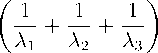
Let us detail the explicit form of the elements of the mixing matrix. First, we take into account that the parametrization of possible values of the mass parameters Mi = — can be λi simplified. Recall that the roots λi are solutions of the characteristic equation

+d 1L1 (M-M2)(M-M3)+d2L2(M-M3)(M-M1)+ A3 - (c 1 + c2)A2 + (c 1 c2 + a2 + b2)A - (c 1 a2 + c2b2) = 0,

+d3L3(M - M1)(M - M2) +

+(M - M 1)(M - M2)(M - M3) = 0.

Given the relation M i = M/A i , the equation can be transformed into the following form

where c ₃ = b >  0 , c 4 = a >  0 . Taking into account the identities

A1 + A2 = c1 + c2 - A3 ,

c 1 a ² + c 2 b ²

^A 1 ^A 2 =-----7------ ,

λ 3

-Ц 3 +

M3

λ 1     λ 2

+ L 1 d 1 + L 2 d 2 +

we find expressions for A 1 , A ₂ in terms of A ₃ :

λ 1

^c 1 ⁺ c 2 ^{- A} 3

^{+ L} 3 ^d 3 Ц ^{2 +}

-ML 1 d 1 ^2 - Al - A_

-

c1 + c2 - A3

-

c 1 a ² + c ₂ b ² λ 3

-ML 2 d 2 ^2 — a— A3^ ^-ML 3 d 3 ^^{2 -} a— a2

A2 =

-M ²

+

- 3 M ² + 2 M ²

-

^c 1 ^{+ c} 2 ^{- A} 3 +

+

1 1 1 1 1 1 1 1

λ ₁ λ ₂ λ ₁ λ ₃ λ ₂ λ ₃

c 1 + c 2 - A 3

-

c 1 a ² + c ₂ b²

λ ₃

ц+

M ² L 1 d 1 (1 - ¹ ) (1 - ¹ ) + λ 2          λ 3

+M2 L 2 d 2 ^1 - — ^1 -    +

λ 3          λ 1

⁺ M ² L 3 d 3 f¹ — — f¹ — — ⁺ λ 1          λ 2

The value of the root λ 3 may be arbitrary, because the physically meaningful parameter is M ₃ = M/A ₃ (at an arbitrary M ). The simplest expression for λ 3 is obtained when c 1 = c ₂ = 1 . In this case, the cubic equation is simplified

A3 - 2 A2 + (1+ k) A - k = 0,  k = a2 + b2.

Its roots are given by the formulas

A 3 = 1, A1 = 2 - ^ V1 - 4 k,

A2   2 + 2 —1  4k,  k 6 (0’ 4) '                  M2   1 + vT—4k ’  k 6 (0’ 4) ' Accordingly, the mass parameters Mi are specified by the formulas                                                       Let us construct tables of values for Ai and A-1 = M = M M =    2 M                Mi/M, i = 1,2, (A 3 = A -1 = 1), depending on the 3      ,     1   1 — — 1 — 4 k’             parameter k: Table 1 Parameter values λi = 12 1 ∓ 1 - 4k , i = 1, 2 depending on k Таблица 1 Значения параметров λi = 12 1 ∓ 1 - 4k , i = 1, 2 в зависимости от k k 0.24 0.22 0.209 0.207 0.205 0.203 0.20 0.16 0.12 0.08 0.04 0.01 λ1 0.4 0.327 0.298 0.293 0.288 0.283 0.276 0.2 0.139 0.088 0.042 0.01 λ2 0.6 0.673 0.702 0.707 0.712 0.717 0.724 0.8 0.861 0.912 0.958 0.989 Parameter values Ai 1 =2 (1 y V1 _ 4k) 1, i = 1, 2 depending on k Значения параметров A-1 =2 (1 y V1 _ 4k) 1, i = 1, 2 в зависимости от k Table 2 Таблица 2 k 0.24 0.22 0.209 0.207 0.205 0.203 0.20 0.16 0.12 0.08 0.04 0.01 1 /A 1 2.5 3.058 3.356 3.413 3.472 3.534 3.623 5 7.194 11.364 23.810 100 1 /A 2 1.667 1.486 1.425 1.414 1.404 1.395 1.381 1.250 1.161 1.096 1.044 1.011 where

Let us detail the coefficients L _i in the expression for

Ф( x ) :

Ф( X ) = L 1 Ф 1 ( X ) + L 2 Ф 2 ( x ) + L з Ф з ( x ) ,

L = 1 + —6, (a2 + b2) = k

< 4 , 0 <  2 ь <  1 .

- 2 k        1

b (A i — A 2)( A i — A 3)

+ 11 — 2( A 2 + A 3) + 4 A 2 A з 2 Lb (A i — A 2)(A i — A 3)

Let us detail the coefficients d i :

- 4Bb d1 = 6M P1

—

11 , d2

2 ) ’      2

4Bb

6M v 2

—

1A

I/ ’

d 3

—2 k        1

b (A 2 — A 3)(A 2 — A1)

+  1 1 — 2(A 3 + A 1)+4 A 3 A1

+ 2Lb (A 2 — A 3)(A 2 — A1)

4Bb

6M v 3

—

.

Combinations d i L j appear in the mixing matrix, so the parameter b in the denominators in (10) will be canceled with the parameter b in (11). Also, since the dimension of the quantity B is M ² (inverse square meter), we can introduce substitutions

—2 k        1

b (A 3 — A 1)( A 3 — A 2)

1 1 — 2( A1 + A 2)+4 A1A 2

2 Lb (A 3 — A1)(A 3 — A 2)

or (we take into account that A ₃ = 1 )

L1 =

1            1

b (A1 — 1)(A1

— A 2)

— 2k + 2L ( — 1 + 2A2)

4B = 6rM2 ^ d = M-B^bA, — 1) =

i    6 M2 V 2/

= Mrb ^Ai — I) = MDi, where the quantities Di are dimensionless. With this in mind, the cubic equation (9) is transformed to the form

L 2 ⁼

-----—---- X

b (A2 — 1)(A2 — A1)

—ц3 + M 3 — — — — — a—+ L1D1 + L 2 D 2+

L3 =

X

X

—2 k + 2L(—1 + 2 A1)

-------—------ X

b (1 — A 1)(1 — A2)

—2 k + 2L(1 — 2 A1

— 2A2 + 4A1A2)

+ L 3 D 3 ц ² + M ²

—L 1 D 1 (2 —

λ 2

—

λ 3

—

—L2 D2 ^2 — A11 — A13) — L3 D3 (2 — A11 —

—

1 λ2

— 3+2

—

11 + 11 + 11

λ ₁ λ ₂     λ ₁ λ ₃    λ ₂ λ ₃

^ ⁺

+ M ³

> 1)⁺

⁺ L ² D ² (1 - У (1 ^—

Since the parameter b enters as a multiplier into D 1 , D 2 , D 3 and the denominators of the expressions for the coefficients L 1 , L 2 , L 3 , then in combinations

L ₁ D ₁ + L ₂ D ₂ + L ₃ D ₃ , L ₁ D ₁ , L ₂ D ₂ , L ₃ D ₃

this parameter is reduced. With this in mind, we have the identities

L 1 ⁼

⁽ > 1 ^{— 1)(} >  1 ^— >  2 )

^{— 2} k ⁺ 2 L ⁽² >  2 ^—

⁺ L ³ D ³ (1 ^- у с ^-

> 2)⁺

= 0 .

L 2 ⁼

( > 2 — 1)( >  2 — >  1 )

^{— 2} k ⁺ 2 L ⁽² >  1 ^— 1)

The roots of this equation can be found in the form ^ i = M A i , where A i are dimensionless quantities; then the equation for A ₁ , A ₂ , A ₃ takes the form

— A ³ + 3 — >— >— > —+ L i D i + L 2 D 2 + L з D 3 A ² +

+ —L 1 D 1 ^2 — >— ^ —L 2 D 2 ^2 — —

—

λ 3

—

^—L ^{3 D 3} (^{2 —} ■ 1 1 ^— > 1 2) ^{— 3 + 2} (£⁺ 1 2 ⁺ ^

³     (1 — >  1 )(1 — >  2 )

x |^{— 2} k ⁺ 2 L ^{(1 —}

^D 1 = 2⁽² > 1 ^— 1) , D 2 = where

> 1 = 2 (1 — V 1 — 4 k ) , k ^ f 1 , 4 j , L = 1 + v

2 > 1 — 2 > 2 +4 > 1 > 2 ) j ,

2(2 >  2 — 1) , D 3 = 2 ,

> 2 =2 (1 + V 1 — 4 k ) ,

=, ( a ² + b ² ) = k <  2

6 v '           4

—

1 1 I 1 1 I 1 1 λ 1 λ 2 λ 1 λ 3 λ 2 λ 3

A+

+ L _i D _i

Also, we should take into account the identities

2 >  ₁ — 1 = — V1 — 4 k, 2 >  ₂ — 1 = +V1 — 4 k, >  ₁ — >  ₂ = —V 1 — 4 k, >  ₂ — >  ₁ = + V 1 — 4 k,

> 1 + >  2 = 1 , >  1 — 1 = —> 2 , >  2 — 1 = —> 1 ,

^{+ L} 2 ^D 2 (1 ^— У (1 ^— £)⁺

^{+ L} 3 ^D 3 ( ^{1 —} .   ( ^{1 —} .   ⁺

λ ₁          λ ₂

1 — 2 >  1 — 2 >  2 +4 >  1 >  2 = 4 k — 1 , >  1 >  2 = k,

then we get simpler expressions

L 1 ⁼

L 2 ⁼

(1 + V 1 — 4 k ) V 1 — 4 k 2

— 2 k + 2 L V 1 — 4 k I ,

Allow for that > ₃ = 1 , then we get

(1 + V 1 — 4 k ) V 1 — 4 k

L ³ = k { ^{— 2} k ⁺2 L

2 k + 2 L V 1 — 4 k \ ,

A ³ + 2 — >> —+ L 1 D 1 + L 2 D 2 + L 3 D 3 A ² +

+

L 1 D 1 ^1 — — + L 2 D 2 ^1 — — +

+ L 3 D 3 (2 —   — ^)+3 — 2(^ + ^ + 1) +

λ ₁     λ ₂               λ ₁     λ ₂

^D 1 = ^— - V ^{1 — 4 k}, ^D 2 = ⁺“ V ^{1 — 4 k},  ^D 3 = -,

L = ^{1 + V} 6 , ⁰ < ^b<  2 .

In this way, we arrive at the following cubic equation for A :

A ³ + A A ² + B A + C = 0 ,

11   1   1

λ 1 λ 2     λ 1     λ 2

A —

where the coefficients are (take into account the properties of the roots λ 1 , λ 2 )

A = ^{2 —} k ^{+ L} 1 ^D 1 ^{+ L} 2 ^D 2 ^{+ L} 3 ^D 3 ,  C = ^L 3 ^D 3 ,

B — -L 1 D 1

-

L 2 D 2

1 - 71 - 4 k

1 + 71 - 4 k

1 + 71 - 4 k

1 - 71 - 4 k

-

+ L3D3 2

-

г +1. k

we obtain

2k

A3 +

-

k

1 A2+

Using identities

+

1+ 1

6   1 - 4k

-

.       2 k - l71 - 4 k

LiDi — ------. r,

1 + 71 - 4 k

, _    2k + l71 - 4k

L2D2 — ------, r,

2 2     1 - xl 4k

2(V6 + b) 2 k

) r A+

6   1 - 4 k

+ l1+2( 76 + b 2 k

) r — 0, (12)

L 3 D 3 —

-

1 - 4k

1 + l — )r'

we transform the cubic equation to a simpler form

2k

A3 +

-

k

1 A2

+ 1+1

-

l1 - 4 k 2 k

r A+

where

0 < k < 4, 0

For definiteness, we set b 1 — 0 , b 2 — 1 , b 3 — 2 . The pa-

rameter r was introduced by the relation 4 B

6 rM 2

1 - 4k

+ 1+ l "ЙГ r — 0.

Allowing for the expression for the parameter l :

l — TL

2(^6 + b)’

from physical considerations, we will assume that the dimensionless parameter r is small. Below we will follow several situations r — 10 ^{_ 5} , r — 10 ^{_ 3} , r — 1 . The last value |r| — 1 corresponds to a very strong magnetic field. Numerical study showed that dependence of the roots A i upon parameter b G (0 , 2) is very insignificant. By this reason below we take the value b — 0 . Let us construct tables of values for the roots A i , A 2 , A 3 equations (12) (see tables 3-5).

Table 3

Таблица 3

Значения корней Д i , i = 1 , 2 , 3 уравнения (12) для b = 0 , r = 10 ⁵

The values of the roots Д i , i = 1 , 2 , 3 of equation (12) for b = 0 , r = 10 ⁵

k	0.24	0.22	0.208	0.204	0.20	0.16	0.10	0.06	0.02	0.01
A i	0.667	0.485	0.419	0.400	0.382	0.250	0.127	0.069	0.021	0.010
A 2	1.500	2.060	2.389	2.502	2.618	3.999	7.873	14.598	47.979	97.990
A 3	-0.00001	-0.00001	-0.00001	-0.00001	-0.00001	-0.00002	-0.00002	-0.00004	-0.00012	-0.00024

Table 4

The values of the roots Д i , i = 1 , 2 , 3 of equation (12) for b = 0 , r = 10 ~ ³

Таблица 4

Значения корней Д i , i = 1 , 2 , 3 уравнения (12) для b = 0 , r = 10 ³

k	0.24	0.22	0.208	0.204	0.20	0.16	0.12	0.08	0.04	0.01
A i	0.670	0.487	0.420	0.401	0.384	0.252	0.164	0.099	0.049	0.021
A 2	1.489	2.059	2.388	2.502	2.617	3.999	6.171	10.404	22.957	97.990
A 3	-0.001	-0.001	-0.001	-0.001	-0.001	-0.002	-0.002	-0.003	-0.005	-0.012

Finally, with an even greater increase in the parameter r , the roots become complex-valued

Table 5

Таблица 5

The values of the roots Д i , i = 1 , 2 , 3 of equation (12) for b = 0 , r = 1

Значения корней Д i , i = 1 , 2 , 3 уравнения (12) для b = 0 , r = 1

k	0.24	0.209	0.206	0.203	0.18	0.12	0.06	0.01
A i	1.265+1.129i	1.588+0.726i	1.625+0.656i	1.662+0.574i	1.173	0.695	0.503	0.406
A 2	-0.362	-0.392	-0.395	-0.398	2.804	6.128	14.727	98.221
A 3	1.265-1.129i	1.588-0.726i	1.625-0.656i	1.662-0.574i	-0.422	-0.489	-0.653	-0.627

This means that at such magnetic field, the model becomes non-interpretable.

Conclusions

In the present paper, the model of a fermion with three mass parameters is studied in presence of the external uniform magnetic field. After diagonalizing transformation, three separate equations are obtained effectively for particles with different anomalous magnetic moments. Their exact solutions and generalized energy spectra are found. After diagonalizing the mixing matrix, we reduce the problem for three separated Dirac–like equations for particles with different anomalous magnetic moment. It is shown that for a very strong magnetic field, the model becomes non-interpretable, because the effective anomalous moments turns out to be complex-valued.