Forecasting of dry freight index data by using machine learning algorithms

Published Online August 2019 in MECS

Maritime transportation plays an important role in the global trade system. Mari-time statistics open a window to global economic actions because overseas trading is too much. Lloyd data presents the shipping prices of bulk cargoes that is generated from daily reported fixtures or estimations of the Baltic Exchange. It is generally hard to forecast these indexes because they are volatile, complex, and cyclic [1]. The prediction of the trend of dry bulk market becomes difficult since the affecting factors of price of dry bulk market are complexities [2].

Lloyd's data includes of the world's largest dedicated marine and energy data. This database consists of the Baltic Dry Index (BDI), Baltic Capesize Index (BCI), Baltic Panamax Index (BPI), and Baltic Supramax Index (BSI) values, updated daily. These indexes project the volatility of dry bulk shipping market and demonstrate the status of the global economy and trend of international trade. They are called as the “barometer” of dry bulk shipping market. Many investors and experts have tried to forecast the future trend of dry bulk shipping market. These indexes are useful for them in order to set their investment portfolio and management risk strategy [3]. BDI, a powerful tool for shipping industry, has been the average of BCI, BPI and BSI since 2006. It reflects bulk shipping market sentiment as a price reference for transaction platform of bulk shipping companies and investors [4].

The aim of this study is to investigate the performance of machine learning algorithms and find the most successful model for analysis of freight index data. In this con-text, the analysis of Lloyd data is performed by utilizing Gradient Boosted Trees (GBT) and Multi-Layer Perceptron (MLP) learning algorithms which are introduced in [5,6] respectively. These algorithms are suitable for nonlinear time-series prediction. By sending the training data as input to these algorithms, supervised machine learning is performed. The performance of prelearned classifier algorithm is tested on the testing data. And so, knowledge discovery is carried out through the data. The BSI out of all data are collected from March 2009 to January 2018. BSI data is collected from August 2012 to January 2018. Eight datasets from Lloyd data are obtained within the frame of two scenarios: a) the last three index values in the freight index datasets (four datasets); b) the last three index values in both crude oil price and freight index datasets (four datasets).

This paper is organized as follows. Section 2 reviews the studies on the shipping freight market. Section 3 introduces the data collection. Section 4 presents performance evaluation criteria. The designed models are introduced in Section 5. The performances of the models are compared and analysed in Section 6. Finally, the conclusion is presented in Section 7.

• II.    Related Work

There are many studies on analysis of freight index data. Şahin et al. [1] introduced an artificial neural network approach for BDI forecasting. According to their studies, the ANN is a considerable method for modelling and forecasting of BDI. Han et al. [2] presented the improved support vector machine model which is combined model of wavelet transform and support vector machine in order to forecast dry bulk freight index. Wong [4] introduced that Autoregressive integrated moving average fits better than Fuzzy heuristic model for the prediction of BDI in their studies. Ming-Tao Chou [7] applied fuzzy time series model to forecast the BDI. According to their studies, the fuzzy time series model is suitable for the BDI’s prediction and better than other models. Giannarakis et al. [8] investigated the effect of economic leading indicator of Baltic dry index on stock returns of socially responsible stock index. According to their studies, BDI affect positively Dow Jones sustainability index world. Geman and Smith [9] aimed to describe and explain the key features of shipping markets; and analyse the behaviour of freight rates. Tsioumas et al. [10] aimed to enhance the forecasting accuracy of the BDI by means of developing a multivariate Vector Autoregressive model with exogenous variables. The model incorporates the Chinese steel production, the dry bulk fleet development and a new composite indicator, the Dry Bulk Economic Climate Index. Ruan et al. [11] investigated the cross-correlation properties of BDI and crude oil prices, using cross-correlation statistics test and multifractal detrended cross-correlation analysis. They verified that the multifractality of the cross-correlations of BDI and crude oil prices are both attributable to the persistence of fluctuations of time series and fat-tailed distributions. Baltyn [12] aimed to identify the level of diffusion index changes between United States Gross Domestic Product and the BDI for different periods of time which are 90 days. Zeng et al. [13] proposed Empirical Mode Decomposition for forecasting of BDI. For this, they decomposed the BDI into three distinct components representing short-term changes, long-run trends, and external shocks respectively. Bao et al. [14] presented a new BDI forecasting model based on Support Vector Machine combined with Correlation-based Feature Selection and introduced the macroeconomic fundamental indicators of BDI. Apergis and Payne [15] disclosed the importance of the BDI in predicting the future course of the real economy, yielding a link between financial asset markets and the macro economy. Yang et al. [16] developed a model which is combination of the wavelet transforms and support vector machine in order to forecast the BPI. Yuwei et al. [17] proposed a model which includes empirical evaluations in order to analyse the leverage effect among the Handysize, Supramax, Panamax and Capesize index in the dry bulk shipping market. As can be seen, there are very studies which were performed, using BDI data, while there are few studies which were carried out, using other indexes. Even though BDI is expressed as the average of these four indexes, the contribution of this study to the literature is conducted by focusing on each of them separately in this study.

• III.    Data Collection

  Lloyd data which were gathered from Quandl offers the BDI, BCI, BPI and BSI values updated daily. Quandl's data contain various objects including timeseries and tables. Researchers can access the premium data through the APIs and various tools. Also, the crude oil price (COP) data are collected from the Federal Reserve Economic Data (West Texas Intermediate (WTI) - Cushing, Oklahoma). The information about the daily index data is given in Table 1. For example, the timeseries of BSI consist of data between August 2012 and January 2018. The sample size, weekly average value, is 280 for this dataset.

Table 1. The data range for daily index data.

	Time Interval
Datasets	Start Date	End Date
BCI	2009-03-16	2018-01-28
BPI	2009-03-16	2018-01-28
BDI	2009-03-16	2018-01-28
BSI	2012-08-21	2018-01-28
COP	2012-08-21	2018-01-28

First, the weekly average values are obtained from the daily index data. This information is presented in Table 2 in detail. For example, there are 456 records for BDI. The 319 prior consecutive records are assigned as the training set, and the last 137 records are assigned as the testing set.

Table 2. Weekly average data for datasets.

Datasets	Start Date – End Date	Total size	Train size	Test size
BPI	Week 13,2009 - Week 4,2018	456 weeks	319 weeks	137 weeks
BPI	Week 13,2009 - Week 4,2018	456 weeks	319 weeks	137 weeks
BDI	Week 13,2009 - Week 4,2018	456 weeks	319 weeks	137 weeks
BSI	Week 35,2012 - Week 4,2018	280 weeks	196 weeks	84 weeks
COP	Week 35,2012 - Week 4,2018	280 weeks	196 weeks	84 weeks

• IV.    Performance Evaluation

To assess the performance of the learning algorithm, it is determined how well the method produces estimates that match the actual results. Mean Absolute Error (MAE), Root Mean Squared Error (RMSE) and R-squared (R2) evaluation metrics which are expressed respectively by the following equations are used in order to assess the prediction accuracy of the models.

MAE=

n n 1 s |ei| i=1

1/2

RMSE= n ^-1 Z |e j              (2)

_    i=1     _ where ei is defined as individual model prediction error usually (ei=Pi–Oi). n is the number of data samples, Pi and Oi are the predicted and observed values respectively in these equations [18].

n

.Z (y-y)2

R2=1-i=1                      (3)

ⁿ Z (y-y)² i=1

where y is the observed response variable, y its mean and yˆ is the corresponding predicted values. R2, commonly used in statistics and also known as the coefficient of determination, is a measure of how well a model fits a dataset. It measures the degree of variation in the target variable; this is explained by the variation in the input features. This coefficient generally takes a value between 0 and 1, where 1 equates to a perfect fit of the model [19].

• V.    Designed Models

This study basically consists of three stages:

• 1.    Preparation of data for each freight index.

• a.    The datasets which include weekly average Lloyd values as time-series are obtained.

• b.    The whole data normalized by using min-max normalization technique in order to avoid the training and prediction error.

• 2.    Preparation of datasets within the frame of the past observations.

• a.    Past observations in t-2, t-1 and t times.

• b.    Past observations included COP data in t-2, t-1 and t times.

• 3.    The Designed Models for Lloyd Data Prediction

• A. Model 1 (1^st approach)

The last two freight index values in t-2 and t-1 times are used as an input parameter. The output parameter is the datum in t time for each freight index.

BDI dataset

Input parameters are BDI(t-2) and BDI(t-1), and output parameter is the BDI(t). The sample size as weekly average data is 456. The portion of the 70% of dataset, prior consecutive data of 319 weeks in between Week 13, 2009 to Week 21, 2015 is reserved for training. The remained portion of dataset, data of 137 weeks in between Week 22, 2015 to Week 4, 2018 is reserved for prediction.

BPI dataset

Input parameters are BPI(t-2) and BPI(t-1), and output parameter is the BPI(t). The sample size as weekly average data is 456. The portion of the 70% of dataset, prior consecutive data of 319 weeks in between Week 13, 2009 to Week 21, 2015 is reserved for training. The remained portion of dataset, data of 137 weeks in between Week 22, 2015 to Week 4, 2018 is reserved for prediction.

BCI dataset

Input parameters are BCI(t-2) and BCI(t-1), and output parameter is the BCI(t). The sample size as weekly average data is 456. The portion of the 70% of dataset, prior consecutive data of 319 weeks in between Week 13, 2009 to Week 21, 2015 is reserved for training. The remained portion of dataset, data of 137 weeks in between Week 22, 2015 to Week 4, 2018 is reserved for prediction.

BSI dataset

Input parameters are BSI(t-2) and BSI(t-1), and output parameter is the BSI(t). The sample size as weekly average data is 280. The portion of the 70% of dataset, prior consecutive data of 196 weeks in between Week 35, 2012 to Week 21, 2016 is reserved for training. The remained portion of dataset, data of 84 weeks in between Week 22, 2016 to Week 4, 2018 is reserved for prediction. B. Model 2 (2^nd approach)

COP data is included to the input parameters dataset. That is, the last two freight index data and COP data in t-2 and t-1 times are selected for input parameter. The output parameter is the datum in t time for each freight index.

BDI_COP dataset

Input parameters are COP(t-2), BDI(t-2), COP(t-1) and BDI(t-1), and output parameter is the BDI(t).

BPI_COP dataset

Input parameters are COP(t-2), BPI(t-2), COP(t-1) and BPI(t-1), and output parameter is the BPI(t).

BCI_COP dataset

Input parameters are COP(t-2), BCI(t-2), COP(t-1) and BCI(t-1), and output parameter is the BCI(t).

BSI_COP dataset

Input parameters are COP(t-2), BSI(t-2), COP(t-1) and BSI(t-1), and output parameter is the BSI(t).

The clauses established for training and prediction information in Model 1 are not included to this section in order to avoid repeated statements.

• VI.    Results

Training sets are sent to the GBT and MLP one by one. After that, test sets are sent to the pre-learning models. So, the learning and prediction successes of these algorithms are evaluated. Our proposed models predicted quite close values to the actual values on the datasets. These results indicate that the actual and the predicted values are consistent with each other. Prediction results of the models and actual values of the datasets based on Model 1 approach are plotted in between Fig. 1 and Fig. 4. Besides, prediction results of the models and actual values of the datasets based on Model 2 approach are plotted in between Fig. 5 and Fig. 8.

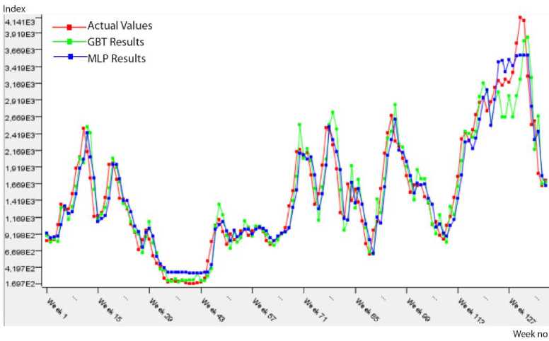
Fig.1. Predicted results on the BCI testing data.

The predicted results approximately same to actual values in Fig. 1 show that performances of the prediction algorithms are close to each other. In addition, Table 3 presents the performance measures of two prediction algorithms within the frame of 1st approach (Model 1). According to this table, the most suitable model for BCI data is MLP because of the minimum error (RMSE: 0.06, MAE: 0.047) and the perfect fit of R2 value (0.926).

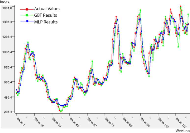
Fig.2. Predicted results on the BPI testing data.

Table 3. Performance results of the algorithms on the BCI testing data.

		Prediction Algorithms
Datasets	Performance Measure	GBT	MLP
BCI	R2	0.894	0.926
	MAE	0.053	0.047
	RMSE	0.072	0.06
Note: Best performances are bolded.

The predicted results approximately same to actual values in in Fig. 2 show that performances of the prediction algorithms are close to each other. In addition, Table 4 presents the performance measures of two prediction algorithms within the frame of 1st approach (Model 1). According to this table, the most suitable model for BPI data is GBT because of the minimum error (RMSE: 0.072, MAE: 0.049) and the perfect fit of R2 value (0.923).

Note: Best performances are bolded.

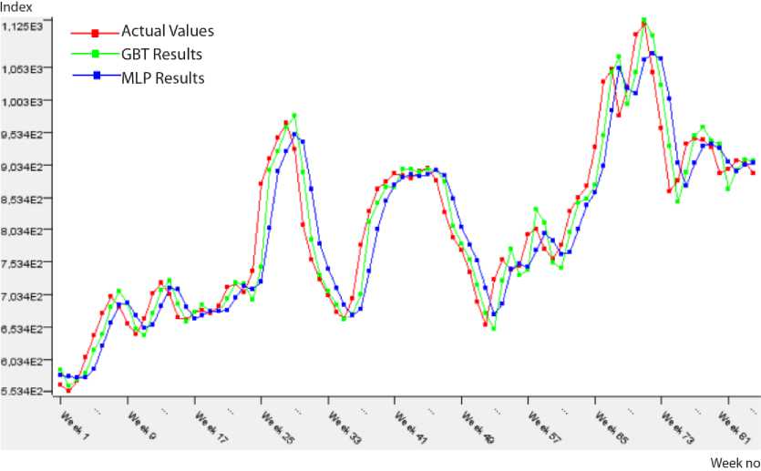
Table 4. Performance results of the algorithms on the BPI testing data.

		Prediction Algorithms
Datasets	Performance Measure	GBT	MLP
BPI	R2	0.923	0.891
	MAE	0.049	0.064
	RMSE	0.072	0.086

Fig.3. Predicted results on the BSI testing data.

The predicted results approximately same to actual values in Fig. 3 show that performances of the prediction algorithms are close to each other. In addition, Table 5 presents the performance measures of two prediction algorithms within the frame of 1st approach (Model 1). According to this table, the most suitable model for BSI data is GBT because of the minimum error (RMSE: 0.063, MAE: 0.047) and the perfect fit of R2 value (0.921).

The predicted results approximately same to actual values in Fig. 4 show that performances of the prediction algorithms are close to each other. In addition, Table 6 presents the performance measures of two prediction algorithms within the frame of 1st approach (Model 1). According to this table, the most suitable model for BDI data is GBT because of the minimum error (RMSE: 0.051, MAE: 0.041) and the perfect fit of R2 value (0.952).

Table 5. Performance results of the algorithms on the BSI testing data.

		Prediction Algorithms
Datasets	Performance Measure	GBT	MLP
BSI	R2	0.921	0.86
	MAE	0.047	0.066
	RMSE	0.063	0.084

Note: Best performances are bolded.

Table 6. Performance results of the algorithms for Model 1 approach.

		Prediction Algorithms
Datasets	Performance Measure	GBT	MLP
BDI	R2	0.942	0.952
	MAE	0.042	0.041
	RMSE	0.056	0.051

Note: Best performances are bolded.

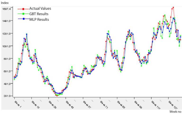
Fig.4. Predicted results on the BDI testing data.

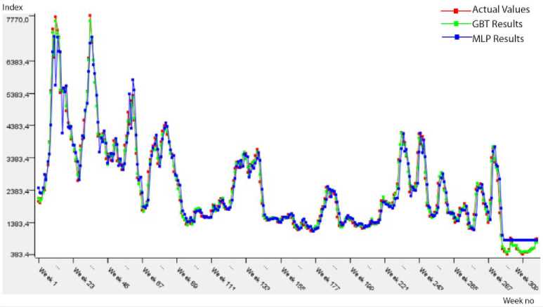
Fig.5. Predicted results on the BCI_COP testing data.

The predicted results approximately same to actual values in Fig. 5 show that performances of the prediction algorithms are close to each other. In addition, Table 7 presents the performance measures of two prediction algorithms within the frame of 1st approach (Model 2). According to this table, the most suitable model for BCI_COP data is MLP because of the minimum error (RMSE: 0.065, MAE: 0.052) and the perfect fit of R2 value (0.913).

Table 7. Performance results of the algorithms for Model 2 approach.

Datasets	Performance Measure	GBT	MLP
BCI_COP	R2	0.906	0.913
	MAE	0.052	0.052
	RMSE	0.067	0.065

Note: Best performances are bolded.

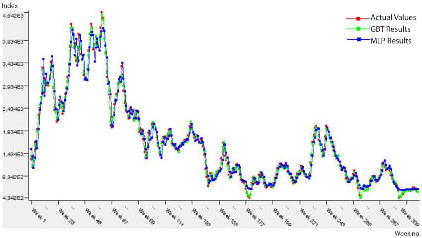
Fig.6. Predicted results on the BPI_COP testing data.

The predicted results approximately same to actual values in Fig. 6 show that performances of the prediction algorithms are close to each other. In addition, Table 8 presents the performance measures of two prediction algorithms within the frame of 1st approach (Model 2). According to this table, the most suitable model for BPI_COP data is MLP because of the minimum error (RMSE: 0.074, MAE: 0.057) and the perfect fit of R2 value (0.918).

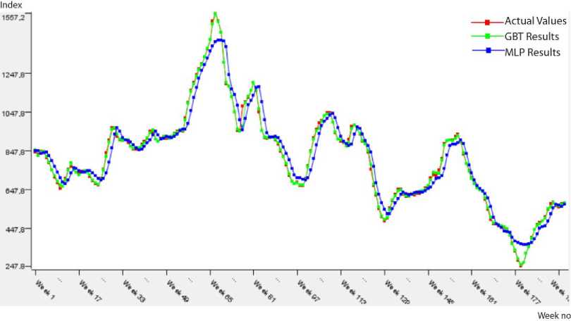
Fig.7. Predicted results on the BSI_COP testing data.

Table 8. Performance results of the algorithms for Model 2 approach.

Datasets	Performance Measure	GBT	MLP
BPI_COP	R2	0.911	0.918
	MAE	0.058	0.057
	RMSE	0.077	0.074

Note: Best performances are bolded.

The predicted results approximately same to actual values in Fig. 7 show that performances of the prediction algorithms are close to each other. In addition, Table 9 presents the performance measures of two prediction algorithms within the frame of 1st approach (Model 2). According to this table, the most suitable model for BSI_COP data is GBT because of the minimum error (RMSE: 0.079, MAE: 0.059) and the perfect fit of R2 value (0.878).

Table 9. Performance results of the algorithms for Model 2 approach.

Datasets	Performance Measure	GBT	MLP
BSI_COP	R2	0.878	0.747
	MAE	0.059	0.085
	RMSE	0.079	0.114

Note: Best performances are bolded.

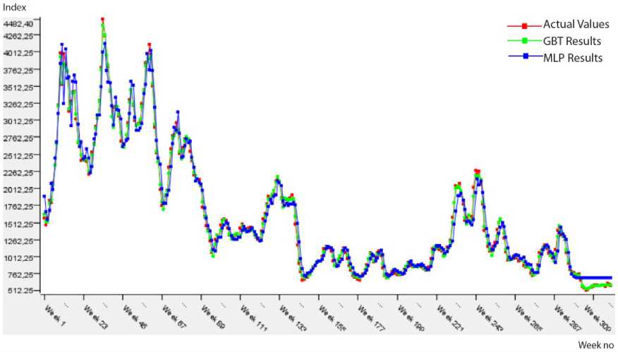
Fig.8. Predicted results on the BDI_COP testing data.

The predicted results approximately same to actual values in Fig. 8 show that performances of the prediction algorithms are close to each other. In addition, Table 10 presents the performance measures of two prediction algorithms within the frame of 1st approach (Model 2). According to this table, the most suitable model for BDI_COP data is MLP because of the minimum error (RMSE: 0.054, MAE: 0.042) and the perfect fit of R2 value (0.947).

Table 10. Performance results of the algorithms for Model 2 approach.

Datasets	Performance Measure	GBT	MLP
BDI_COP	R2	0.933	0.947
	MAE	0.044	0.042
	RMSE	0.06	0.054
Note: Best performances are bolded.

• VII.    Conclusion

Maritime transportation highly affects the global economic system due to overseas shipping too much. Lloyd data presents the shipping prices of bulk cargoes that are generated from daily reported fixtures or estimations of the Baltic Exchange. Forecast of these index generally is hard because they are volatile, complex, and cyclic. In shipping sector ship owners, ship brokers, operators, traders, etc. depend on their past experience for their future decisions as a rule. Previous studies usually investigate the forecast of BDI data by considering diverse statistical regression methods. In this study, the prediction performances of the models designed with GBT and MLP algorithms are presented for four types of freight index data, Lloyd data. This study investigates the effectiveness of the prediction algorithms for the prediction of all freight index datasets and its applicability. In addition, GBT is the most consistent algorithm for BPI and BSI data. Moreover, MLP is the most convenient algorithm for BCI, BDI and

BPI data while GBT is the most suitable algorithm for BSI data within the frame of 2nd approach. This study could be a powerful and beneficial reference in order to avoid risk in the shipping industry. In the future, the deep neural networks based models will be designed and the performances of these models will be compared.

Acknowledgment

The author is thankful to the Quandl and Federal Reserve Economic Data (West Texas Intermediate (WTI) - Cushing, Oklahoma) for the datasets.