Forecasting Performance of Random Walk with Drift and Feed Forward Neural Network Models

Forecasting is define by Box and Jenkins [1] as a planning tool that aids an organization in its attempts to survive with the uncertainty of the future, trusting mainly on data from the past and present as well as analysis of trends. Forecasting begins with assumptions based on the organization’s experience, knowledge and judgement. These estimates are anticipated into the coming months or years using one or more methods such as Box-Jenkins models, Delphi method, exponential smoothing, moving averages, regression analysis, and trend projection. Since any variation in the assumptions will result in a similar variation in forecasting, the method of sensitivity analysis is used which assigns a range of values to the uncertain variables. A forecast should not be confused with a budget.

Artificial Neural Networks (ANNs) consists of interrelated neurons that maneuver in parallel and linked collectively through weights as defined by Lippman [2]. ANNs have been applied in diverse submissions such as:

pattern classification, image and signal processing as asserted by Ibrahim [3]. Carmichael [4] also asserts that a neural network is comprised of a quantity of nodes allied by links. Each link has a numeric weight related with it. Weights are the key means of long-term storage in the network, and learning takes place by updating the weights. Specific nodes are linked to the outside setting, and can be labeled as input or output nodes. Artificial Neural Networks (ANN) establishes a family of empirical techniques that imitate biological information dispensation. Most animals possess a neural system that treats information. Biological neural structures consist of neurons, which institute a network through synaptic connections amid axons and dendrites. With these connections, neurons converse chemo-electrical motions to institute behavior. An important artificial neural network is the backpropagation neural network (BPNN) which is a multi-layer feed forward ANN. The BPNN is useful only when the network design is taken appropriately. Excessively minor network cannot learn the problem fine, but excessively huge magnitude will transit to over fitting and unfortunate generalization performance [2]. The backpropagation algorithm (BP) can be used to train the BPNN image density but its weakness is slow convergence. Many methods have been supported out to develop the speed of convergence. Image density is a depiction of an image with rarer jiffs to decrease the probability of diffusion errors. Al-Allaf [5] explain that many literatures deliberated the use of diverse ANN designs and training algorithms for image density to advance the speed of convergence and deliver high density ratio (DR). Roy et al. [6] established an edge conserving image density procedure using one hidden layer feed forward BPNN. Edge detection and multi-level thresholding processes are used to decrease the image magnitude. The treated image block is served as a separate input pattern whereas single output pattern has been created from the novel image. Their investigation realized a signal to noise (SNR) of 0.3013 and density ratio (DR) of 30:1 when they experiment their method on Lena image.

Idowu et al.[7] applied artificial neural network to make forecast of stock market in Nigeria, using four different banks. Their results specify a measure of how well the variation in the output as described by the targets is very close to 1 for all the four bank stocks covered, which indicates that the artificial neural network model is a good fit. The precision of their forecast was measured using the notion of relative error and the outcomes were quite due, even though it did not attain 100 percent level of precision. Since artificial neural network are good in predicting stocks of the four banks in Nigeria, it is improbable that an artificial neural network will ever be the perfect forecasting method that is anticipated as the elements in a huge dynamic system like the stock market are too complex to be comprehended overtime.

Bianco et al. [8] asserted that time series forecasting is a prodigious encounter in numerous fields. In finance, one can predict stock exchange courses or indices of stock markets, while data dispensation consultants predict the flow of information on their networks. Globally, energy consumption is intensifying dissolutely for the reason that there is growth in human population, incessant pursuits for healthier living values, prominence on extensive industrialization in undercapitalized countries and the prerequisite to withstand constructive economic evolution charges. Sequel to this fact, a comprehensive forecasting method is vital for correct investment formation of energy generation and distribution. The shared tasks to the growth of dependable forecasts are the resolution of sufficient and necessary information for a respectable prediction. If the information level is inadequate, forecasting will be reduced; likewise, if information is redundant, modeling will be difficult or lopsided. He further stated that it is a well-known fact that complex models gives precise forecasts, but are difficult to accomplish, but simple models gives less accurate forecast and are valued particularly if the forecasting segment is just a measure of an added composite formation device, as frequently is the case.

A mineral resource product which is vital to global economy is crude oil. Strictly speaking, crude oil is a key factor for the economic advancement of industrialized and developing countries as well as undeveloped countries respectively. Besides, political proceedings, extreme meteorological conditions, speculation in fiscal market amidst others are foremost events that characterized the eventful style of crude oil market, which intensifies the level of price instability in the oil markets.

The crude oil industry in Nigeria is the largest industry. Oil delivered around 90 percent of foreign exchange incomes, about 80 percent of federal government proceeds and enhances the progress rate of the country’s gross domestic product (GDP). Ever since the Royal Dutch Shell discovered oil in the Niger Delta in 1956, specifically in Oloibiri, Bayelsa state, the crude oil industry has been flawed by political and economic discord mainly due to a long antiquity of corrupt military governments, civilian governments and collaboration of multinational corporations, particularly Royal Dutch Shell. About six oil firms namely - Shell, Elf, Agip, Mobil, Chevron and Texaco controls the oil industry in

Nigeria. The aforementioned oil companies collectively dominate about 98 percent of the oil reserves and operational possessions. There are three key players in the Nigeria oil industry which include the Federal Ministry of Petroleum Resources, the Nigerian National Petroleum Corporation (NNPC) and the crude oil prospecting companies which comprise the multinational companies as well as indigenous companies as asserted by Baghebo [9].

Singh and Gill [10] asserts that the typical neural network method of executing time series forecasting is to prompt the function say f, by means of every feed forward function approximating neural network architecture, using a set of n - tuples as inputs and a single output as the target rate of the network. They also demonstrated that the hybrid backpropagation genetic method is a standard way to train neural networks for weather forecasts, but shows that the key weakness of this technique is that weather factors were supposed to be independent of each other and their sequential association with one another was not measured. They however, anticipated an improved time series based weather forecast model to exclude the difficulties experienced by the hybrid back propagation / genetic algorithm method.

Nanda et al. [11] in their study predicted estimated rainfall in India using a complex statistical model ARIMA (1,1,1) and three different kinds of artificial neural network models namely multilayer perceptron (MLP),functional-link artificial neural network (FLANN) and Legendre polynomial equation (LPE) in artificial neural network. They used the ARIMA (1,1,1) for the analysis of rainfall estimation data and effectively applied the three artificial neural network models stated before with the complex time series model. Their results revealed that FLANN exhibits very close and better forecasting outcomes as equated to ARIMA model with a low absolute average percentage error (AAPE).

This study intends to provide a comparison study of linear and nonlinear techniques in forecasting the daily crude oil production of the Nigeria National Petroleum Corporation (NNPC). The linear method to be involve here is a random walk with drift model, while the nonlinear model to be involve here is a feed forward neural network model. The forecasting performances of these linear and nonlinear models will be evaluated through the determination of both the root of mean square error (RMSE) and the mean absolute error (MAE).

The remaining part of this study is organized as follows. Section 2 describes the linear and nonlinear methods involve in the study. Section 3 presents simulation results on data obtained from the NNPC for a period of 6 years (2008-2013) using the linear and nonlinear models involved in the study. We report conclusions and future work in section 4.

• II.    Linear and Nonlinear Forecasting Techniques

As we mentioned in section 1, the study will focus on linear and nonlinear techniques to model and forecast the daily crude oil production of the NNPC. These linear and nonlinear techniques are the random walk with drift technique and the feed-forward neural network method respectively. There are numerous comparison investigation using different forecasting methods for predictions. Furundzic [2] presented a comparison study of regression models and neural network models for rainfall-runoff forecasting. Tawfik [3] compared autoregressive models (AR) models and neural network models. Chang et al.[4] presented a comparison of static feed-forward neural network models and dynamic feedback neural network modes. Castellano et al. [5] provided a comparison of autoregressive integrated moving averages (ARIMA) models and neural network models.

Pindyck [6] scrutinizes long-run performance of crude oil, coal, and natural gas prices from 1987-1996 of the organization of petroleum exporting countries (OPEC). He incorporates unobservable formal variables such as minimal costs, the resource reserve base, and request parameters into the model and appraised the model with a Kalman filter. He examines the forecasting capacity of the model, adding mean reversion to a deterministic linear trend. The outcomes propose that the inclusion of a deterministic linear trend creates more accurate forecasts. Radchenko [7] encompasses the Pindyck study. He applies a shifting trend model with an autoregressive procedure in error terms reasonably than Pindyck’s white noise procedure. The outcomes endorse Pindyck’s conclusions. He also states that the shortcoming of the model is an incompetence to reflect the impact of OPEC’s behavior. In view of this purpose, he combines the model with autoregressive and random walk models and completes that the pooled model outperforms the novel model.

Halkos and Kevork [8] showed that when the parameter 6 of an ARIMA (0,2,1) is close to -1, due to the low powers of the Dickey-Fuller (DF) and Augmented Dickey Fuller (ADF) unit root tests, it is very likely to accept that the process of generating the data is the random walk with drift. Aiming therefore to forecast future values of the series, instead of using the real ARIMA (0, 2, 1) model, they used the prediction equation and the error variance of the S -period forecast given by the random walk model.

Grounded on Krycha and Wagner [9], there are about 30 different neural network architectures that have been created, developed, and used so far. A neural network architecture is defined to include several elements: (i) number of input neurons, (ii) number of hidden layers, (iii) number of neurons in each layer, (iv) number of output neurons,(v) transfer function for each neuron, (vi) error function, and (vii) the ways of neural connections.

Maier and Dandy [10] presented a back-propagation (BP) trained feed-forward network modeling monitor, covering data transformation, input variable determination, hidden neuron determination, weight optimization, and model performance authentication. Concerning data transformation, removal of trends and heteroscedasticity is acclaimed. To determine model inputs, either cross-correlation analysis or step-wise approach can be used.

A radial basis function (RBF) network is typically a three-layer network, comprising of an input layer, a hidden layer, and an output layer. The network draws a boundless pact of interest due to fast training and easiness. The hidden layer of the RBF network consists of various neurons that form a parameter vector called center. The center can be measured as the weight vector of the hidden layer. A distance is used to measure how far an input vector is from the center. Hidden neurons use Gaussian functions as activation functions as per Haykin [11] and Sukyens et al. [12].

• A.    Random Walk with Drift

A random walk is defined as a process where the current value of a variable is composed of the past value plus an error term defined as a white noise (a normal variable with zero mean and variance one). Algebraically a random walk is represented as follows:

y_t = У t - 1 + S

The consequence of a procedure of this type is that the best forecast of y for next period is the current value, or in other words the process does not allow predicting the change ( y_t — y_t_ _x) . That is, the transformation of y is unequivocally random. It can be shown that the mean of a random walk process is constant but its variance is not. Therefore a random walk process is nonstationary, and its variance rises with t. In practice, the occurrence of a random walk process makes the forecast process very simple since all the upcoming values of y for s > 0, is simply y_t .

A drift performs like a trend, and the procedure has the following form:

yt = yt—1 + a + S (2)

For a >  0 the process will show an upward trend. This process displays both a deterministic trend and a stochastic trend as explained by Rowland [13].

The random walk with drift will be used as our linear forecasting model. The daily crude oil production data of the NNPC will be first difference in level or in log. Difference series and log difference series are measured as stationary independent increments.

• B.    Feed-forward Neural networks

Neural networks, or artificial neural networks (ANN), are analogous computational models, comprising of interconnected adaptive dispensation units. The dispensation units are named “neurons” and the interconnections are named “networks” as asserted by Sathasivam [14].

In an assertion by Fadare [15] asserts that in a feedforward neural network (FNN), the neurons are congregated into layers. Information drifts from the input layer to the output layer always in one direction; it never goes backwards. There may be middle layers, which are named “hidden layers”. Neurons are linked from one layer to the next, but not inside the same layer. A feedforward neural network is stationary. It performs stationary plotting between an input space and an output space. Fadare [15] further stated that in neural networks, knowledge is acquired during the training or learning process by adjusting the weights in the network through different algorithms. The network weights are improved literarily until the network reproduces the anticipated output from a given set of input. The network is trained with either supervised learning (when both input and the anticipated output are presented to the network) or unsupervised learning (when the anticipated outputs are not used in the training). The back propagation algorithm is a supervised training rule with multiple-layer networks, in which the network weights are stirred along the negative of the gradient of the mean squared error (MSE) so as to minimize the variation among the network’s output and the preferred output.

Neurons in a neural network possessed activation functions which process inputs and produce outputs. The activation function chosen for this study is the activation function of uni-polar sigmoid function given as follow:

f ( X ) = -—— (activation function) (3)

This function is particularly beneficial to use in neural networks trained by back propagation algorithms, since it is easy to differentiate, and this can minimize the calculation capacity for training. The term sigmoid means ‘S’-shape. The net input to neuron j is given by:

nwt. = 2/ wx + 6j (net input function) (4)

where is the output from the previous layer, w is the weight of the node linking neuron i to neuron j, and в • is the bias of neuron j.

j

The target from neuron j is given by:

yj = f ( nwtj •) =---- "^T (neuron target fnc.)

1 + e ^nWj

applying (5)

f / ( nwt ) =

- - ^nwtj

₍ 1 + Г nwtj ) ²

= ^f ( ^nwtj ) ( 1 ^- f ( ^nwtj

■v! =(l -У< )

In terms of the back propagation algorithm, the minimization of the error function is executed by the gradient-descent technique and a weight change is computed as the partial derivative of the error function with respect to each weight w :

ij

Aw = wZi Xi (weight adjusting function) (7) ij j i where w is the learning rate and Z is the error of neuron j.

Shan [16] Levenberg-Marquardt algorithm use the information of the second order derivatives of error terms since the signs of second derivatives of error terms figures out the searching direction of the optimal solution. This algorithm is used here to execute the network training and it has enhanced training at the advanced cost of multifarious computations.

The log difference series performs better in modeling and forecasting greater than the original daily crude oil production series of the NNPC and this assertion shall be illustrated in section 3. Consequently, instead of applying the original series, we will apply the log difference series of the daily crude oil production series of the NNPC.

• III.    Results and Discussion

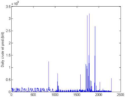
  The data series for this study represents the daily crude oil production of Nigeria National Petroleum Corporation (NNPC). Fig.1 shows the whole picture of 2191 samples for a period of six years (1st January, 2008 - 31^st December, 2013) in barrels per day.

Series number

Fig. 1. Daily Crude Oil Production of the NNPC

The increment series, that is, difference series and log difference series of the daily crude oil production series of the NNPC is used to conduct the Dickey-Fuller (DF) test to determine if the data series is stationary. A sample autocorrelation picture of the daily crude oil production series is shown in fig. 2. The figure points out that the daily crude oil production series of the NNPC are autocorrelated

In this study we difference the original daily crude oil production series by using X_t = Y_t - Y_t__x and Q_t = log ( y ) - log ( y_ J respectively, if Y_t is the original series. Fig.3 shows the picture of the daily crude oil production difference series of the NNPC.

The log difference series of the daily crude oil production is also illustrated pictorially in fig.4. Comparing Figs. 3 and 4 we notice that the log difference series of the daily crude oil production series of the NNPC has a smaller variance than the difference series of the daily crude oil production of the NNPC. The mean value of the difference series is 1.2790e+03, the median value is -11184 and the variance is 3.0162e+14. For the log difference of the NNPC series, the mean value is 0.0028, the median value is and -0.0056 and the variance is 0.3889. The variance of the difference series and log difference series confirms our assertion in figs. 3 and 4

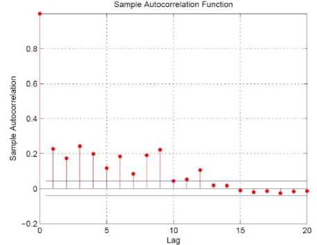
Fig. 2. Autocorrelation Function of the Daily Crude Oil Production series of the NNPC

That the difference series has a greater variance than the log difference series.

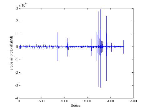
Fig. 3. Daily Crude Oil Production Difference Series of the NNPC

An Augmented Dickey-Fuller (ADF) test of trend stationary is implemented by the MATLAB command “kpsstest” on the difference and log difference series of the daily crude oil production data of the NNPC. The outcome points out that there is no statistical significant indication to accept the null hypothesis that unit roots occur for the difference series and log difference series for the daily crude oil production data of the NNPC. Hence, we conclude that the daily crude oil production difference series and the daily crude oil production log difference series are both stationary.

From the above analogy, one could deduce that the difference series and the log difference series for the daily crude oil production series of the NNPC will give better modeling and forecasting outcomes than the original daily crude oil production series of the NNPC.

In view of this reason, we will use the log difference series only for subsequent analysis, since it has demonstrated that its outcomes will produce better modeling and forecasting results than the difference series.

In this paper, we indicate that for the linear method, that is, the random walk with drift method, forecasting models will be hinge on two input variables, three input variables and four input variables. The procedure also applies to the nonlinear method, that is, the feed-forward neural network method. For both linear and nonlinear models forecasts is made based on four varied sample measurement: 30 data measurements, 90 data measurements, 180 data measurements and 360 data measurements. Furthermore for both linear and nonlinear models, our forecast is hinge on one day, three days and five days ahead predictions. This procedure will now result in the computation of one day, two days and three days ahead root mean square error (RMSE) and mean absolute error (MAE) for each model. This process determines the pattern in which RMSEs and MAEs are at variant from one day to three days predictions and from three days to five day predictions.

Suppose a given set of observations are identically and independently distributed, the forecasts with the smallest mean square error in such observations are the best forecasts. This study evaluates forecasting performances by computing the root mean square error (RMSE) and mean absolute error for the log difference series of the daily crude oil production series of the NNPC.

The computational outcomes for root mean square error (RMSE) and mean absolute error for (MAE) for log difference series of the daily crude oil production series of the NNPC is illustrated in tables 1and 2. It can be seen from the tables that MAEs possessed better forecasting performances than RMSEs, since the values of the MAEs are smaller than the values of the RMSEs, thereby producing the optimal forecasts. Also, in tables 1 and 2, RMSEs and MAEs for two days, three days forecasting are not indispensably at variant with one day forecasting, since the variation is not very significant. The RMSEs and MAEs for the data sample measurements for 30 days, 90 days, 180 days and 360 days for one, three and five days predictions are respectively equivalent. This outcome indicates that the length of the sample data does not necessarily changes the forecasts for varying day’s predictions.

In the feed-forward neural network model we used the concept of stochastic decompositions by Becker [27] to decompose the log difference series into two, three and four independent series. In this study we considered only the four independent series which is used as input variables for the feed-forward neural network model. Table 2 shows the RMSE and MAE forecasting performances for four input variables with one day, three days and five days predictions based on data sample length of 30, 90, 180 and 360 days data samples respectively.

Table 1. Log difference series performance using random walk with drift for root mean square error

Variable Name	RMSE
30 days forecast f1 rmse	0.99561032089558243
30 days forecast f2 rmse	0.80712676029643182
30 days forecast f3 rmse	0.87839236853294578
90 days forecast f1 rmse	0.99561032089558243
90 days forecast f2 rmse	0.80712676029643182
90 days forecast f3 rmse	0.87839236853294578
180 days forecast f1 rmse	0.99561032089558243
180 days forecast f2 rmse	0.80712676029643182
180 days forecast f3 rmse	0.87839236853294578
360 days forecast f1 rmse	0.99561032089558243
360 days forecast f2 rmse	0.80712676029643182
360 days forecast f3 rmse	0.87839236853294578

Table 2. Log difference series performance using random walk with drift for mean absolute error

Variable Name	MAE
30 days forecast f1 rmse	0.64417998499969742
30 days forecast f2 rmse	0.5357206021316514
30 days forecast f3 rmse	0.57357273855963831
90 days forecast f1 rmse	0.64417998499969742
90 days forecast f2 rmse	0.5357206021316514
90 days forecast f3 rmse	0.57357273855963831
180 days forecast f1 rmse	0.64417998499969742
180 days forecast f2 rmse	0.5357206021316514
180 days forecast f3 rmse	0.57357273855963831
360 days forecast f1 rmse	0.64417998499969742
360 days forecast f2 rmse	0.5357206021316514
360 days forecast f3 rmse	0.57357273855963831

In tables 3 and 4 one could see that the MAEs outcomes possessed better forecasting performances than the RMSEs outcomes. This is because the MAEs values are smaller than the RMSEs values, thereby producing the optimal solution. Also, one could see that for the MAEs predictions one day ahead, based on a sample length of 30 days data sample are better than predictions one day ahead, based on a sample length of 90, 180 and 360 days data sample, since MAEs values for one day ahead based on a sample length of 30 days data sample are smaller than one day ahead predictions based on a sample length of 90, 180 and 360 days data samples respectively. This outcome also follow suit for MAEs predictions for two and three day ahead, based on a sample length of 30, 90, 180 and 360 days data samples respectively. The trend for the MAEs is applicable for the RMSEs in that order.

From figs. 1 and 2, one could see that forecasting performances for the nonlinear model, that is, the feed forward neural network model for one day, two days and three days ahead predictions, for data sample length of 30, 90, 180 and 360 days data samples are better than for the linear models, that is, the random walk with drift for one day, two days and three days ahead predictions, for data sample length of 30, 90, 180 and 360 days data samples respectively.

Table 3. Log difference series performance using feed –forward neural network model for root mean square error

Variable Name	RMSE
30 days forecast f1 mae	0.99561032089558243
30 days forecast f2 mae	0.80712676029643182
30 days forecast f3 mae	0.87839236853294578
90 days forecast f1 mae	0.99561032089558243
90 days forecast f2 mae	0.80712676029643182
90 days forecast f3 mae	0.87839236853294578
180 days forecast f1 mae	0.99561032089558243
180 days forecast f2 mae	0.80712676029643182
180 days forecast f3 mae	0.87839236853294578
360 days forecast f1 mae	0.99561032089558243
360 days forecast f2 mae	0.80712676029643182
360 days forecast f3 mae	0.87839236853294578

Table 4. Log difference series performance using feed – forward network model for mean absolute error

Variable Name	RMSE
30 days forecast f1 mae	0.99561032089558243
30 days forecast f2 mae	0.80712676029643182
30 days forecast f3 mae	0.87839236853294578
90 days forecast f1 mae	0.99561032089558243
90 days forecast f2 mae	0.80712676029643182
90 days forecast f3 mae	0.87839236853294578
180 days forecast f1 mae	0.99561032089558243
180 days forecast f2 mae	0.80712676029643182
180 days forecast f3 mae	0.87839236853294578
360 days forecast f1 mae	0.99561032089558243
360 days forecast f2 mae	0.80712676029643182
360 days forecast f3 mae	0.87839236853294578

In view of the foregoing outcome and analogy we assert that nonlinear models have reasonably good performances than linear models in the mean error square sense.

• IV.    Conclusion

This study have shown that nonlinear models have better forecasting performances greater than linear models with regards to the log difference series of the daily crude oil production series of the NNPC. We could deduced from the study that root mean square errors (RMSEs) and mean absolute errors (MAEs) are very stable for very short data lengths such as 30 days data samples as well as with longer data lengths such as 360 days data samples. Speaking firmly on the autocorrelation pattern of the difference series and log difference series of the daily crude oil production of the NNPC series, one could deduce that the daily crude oil production series of the NNPC does not follow a random walk process since the increment series indicates a significant autocorrelation. However, we might ruminate that the daily crude oil production series of the NNPC is a random walk with drift process when one is not trying to predict immediate future values. There have been factors affecting the daily crude oil production of the NNPC such as the Niger Delta militancy unrest which has led to the vandalism of oil pipelines, kidnapping of oil workers, oil theft as well as depriving oil workers access to the oil fields where they work. Future investigation on the daily crude oil production series of the NNPC might consider nonlinear mathematical models of the neural network category with hyperbolic activation functions as well as sine and cosine activation functions to eliminate the irregular factors that affects the daily crude oil production series of the NNPC, such that, a proper spring board will be established upon which models will be developed for forecast.

Acknowledgement

This research is partly financed by Fundamental Research Grant Scheme (203/PMATHS/6711368) from the Ministry of Higher Education, Malaysia and Universiti Sains Malaysia.