Fractional Order EOQ Model with Linear Trend of Time-Dependent Demand

Published Online February 2015 in MECS

• I.    I ntroduction

  Fractional calculus generalizes derivative and integration of a function to non-integer order. This generalization is a rather old problem, as demonstrated by a correspondence, which lasted several months in 1695, between Leibniz and L’Hopital. Many other famous scientists of the past studied and contributed to the development of fractional calculus in the field of pure mathematics[12-16].In recent years the concept of fractional differential calculus has been applied to several fields of engineering, science and economics[5],[6],[10]. Some of the areas where Fractional Calculus has made an important role that are included viscoelasticity and rheology, electrical engineering, electrochemistry, biology, biophysics and bioengineering, electromagnetic theory, mechanics, fluid mechanics, signal and image processing theory, particle physics, control theory[5] and many other field[7], [15]. Only recently, fractional calculus was applied to classical EOQ model to generalize this model in operation research. In a previous paper [4], we have discussed how the fractional calculus can utilizes to develop the classical EOQ model to generalize EOQ model in operation research. In particular, we have seen fractional calculus has a potentiality to apply this concept in any other EOQ model. In this sense we represent the more generalize EOQ model using the broad concept of fractional calculus where demand may vary with time, say linearly instead of constant demand.

The classical EOQ (Economic Order Quantity) [1],[3],[17],[19],[22] model assumes that the demand rate is constant. However, in the real market, [9] the demand for any product cannot be constant. Researchers have paid much attention to inventory modelling with time dependent demand. Silver and Meal [21] developed a heuristic approach to determine EOQ in the general case of a deterministic time-varying demand pattern. Donaldson [8] discussed the classical no-shortage inventory policy for the case of a linear, time dependent demand. This treatment was fully analytical and much computational effort was needed in order to get the optimal solution. Silver [20], using Silver-Meal heuristic obtained an appropriate solution procedure for the case of a positive linear trend in demand to reduce the computational effort needed in Donaldson [8]. Subsequent contributions in this type of modelling came from researchers such as Ritchie ([17],[18]), Kicks and Donaldson [11], and others.

Here we have applied the concept of derivative/integrals with an emphasis on Caputo and Riemann-Liouville fractional derivatives [2],[13] and have some interesting results and ideas[23] that demonstrate the generalized EOQ based inventory model. Fractional derivatives and fractional integrals have interesting mathematical properties that may be utilized to develop our motivation. In this article, first we give a short description on general principles, definitions and several features of fractional derivatives/integrals and then we review some of our ideas and findings in exploring potential applications of fractional calculus in inventory control model.

In section II, we represent a basic conception on Fractional Calculus and short history, description related to Fractional Differential Calculus. In section III, we represent the basic concept of Classical EOQ model. In section IV, we introduce our main work which emphasizes on techniques and procedure for finding our optimum results. Finally, In section V, we present the conclusion of our work.

• II.    A S hort D escription on F ractional D ifferential C alculus

  The origin of fractional calculus goes back to Newton and Leibniz in the seventieth century. S.F Lacroix was the first to mention in some two pages a derivative of arbitrary order in a 700 pages text book of 1819.

He developed the formula for the nth derivative of y=xm , m is a positive integer, ny■  = m xm-n,                    (2.1)

where n( < m) is an integer.

Replacing the factorial symbol by the well-known Gamma function, he obtained the formula for the fractional derivative,

„   , ) = ^{r ( e} ■ 1)    , ^{- a} ,             (2.2)

D x   Г(в - a +1) x

Where a , P are fractional numbers.

In particular he had,

П ^1/2( x ) = П 22  *^/2 = 2 E .            (2.3)

D    Г® ^x   Пл

Again the normal derivative of a function f is defined as, i            f (x + h) - f (x)

D f ( x ) = lim ——'      ,      (2.4)

h ,0         h and

D2f(x)=lim h ,0

f ( x + h ) — t ( x )

This is also valid for non-integer values of n.

Thus on using of the idea (2.8), fractional derivative leads as the limit of a sum given by r          1.     1         <\r      Г(а + 1)              ...  (2.9)

D ^{f ( x} ) = lim y a Z ( - 1)               .^{f ( x - rh} )

h ^ 0 h r = 0        Г ( r + 1) Г ( а - r + 1)

Provided the limit exists. Using the identity

/ ix r Г( а +1)  _ Г( r - a )

(- ) Г(а - r +1) = Г(-а)

(2.10)

The result (2.9) becomes,

D ^ f ( x ) = lim T h -- ZZ Г ( r _:— a ) f ( x - rh )  (2Л1)

h , 0 Г ( - a ) r = 0 Г ( r + 1)

When α is an integer, the result (2.9)reduce to the derivative of integral order n as follows in (2.5).

Again in 1927 Marchaud formulated the fractional derivative of arbitrary order α in the form given by,

D a f ( x ) =

f (x)        a   xx fxx)-f(t), a +         \J         X«+1 dt

^{Г (1 -} a ) x ^{Г (1 a} ) 0 ( x - 1 )

, Where 0<α<1 (2.12)

In 1987, Samko et al had shown that (2.12) and (2.9) are equivalent.

Replacing n by (-m) in (2.7), it can be shown that

0 D -mf (x) = lim hm ZZ h ,0      r=0

m

r

f ( x - rh )

=lim h ,0

f ( x + 2 h ) - f ( x + h ) + f ( x ) h

Iterating this operation yields an expression for the nth derivative of a function. As can be easily seen and proved by induction for any natural number n,

Where

n

Dnf(x) = lim h -n £ (-1)n r=0

I nI к r J

f(x+(n-r)h).

(2.5)

Where

I n ] к r J

n !

(2.6)

Or equivalently,

n

D f ( x ) = lim h ^{- n} Z ( - 1) h , 0       r = 0

1 r In 1 к r J

^{f (} x ^{- rh} )

(2.7)

The case of n=0 can be included as well.

The fact that for any natural number n, the calculation of nth derivative is given by an explicit formula (2.5) or (2.7).

Now the generalization of the factorial symbol (!) by the gamma function allows

I ⁿ 2       n !             Г ( n + 1)

=----------=-------------- (2.8)

к r J   r !( n - r )! Г ( r + 1) Г ( n - r + 1)

J ⁽ x ^- t ^{) ( m} - "f ⁽ t ) dt    ⁽2.13>

( m )₀

m ( m + 1)( m + 2)........( m + r + 1)

r !

(2.14)

This observation naturally leads to the idea of generalization of the notations of differentiation and integration by allowing m in (2.13) to be an arbitrary real or even complex number.

A. Fractional derivatives and integrals

The idea of fractional derivative or fractional integral can be described in another different ways.

First, we consider a linear non homogeneous nth order ordinary differential equation ,

D y = f ( x ), b-X-C                     (2.1.1)

Then {1, x, x2, x3, ........,xn-1} is a fundamental set the corresponding homogeneous equation Dn y=0. f(x) is any continuous function in [b,c], then for any a G (b,c),

y⁽x)= x ⁽ x t )i f ( t ) ^dt a ( n - ^1)!

(2.1.2)

is the unique solution of the equation (2.1.1) with the

initial data

( k )

y (a)=0,

for 0 ≤ k ≤ n - 1 . o r equivalently,

^x             n - 1

=   ¹     ( x - t )   f ( t ) dt

Γ ( n ) ₀

∴ y(x)= ₀ D ^- _x ⁿ f ( x )

(2.1.8)

y(x)= D ^{- n} f(x)=   ^{1 x} ( x - t ) ^{n - 1} f(t)dt  (2.1.3)

a x      Γ(n)

= L ^{- 1}{ s ^{- n} f ( s )} =   ^{1 x} ( x - t ) ^{n - 1} f ( t ) dt

Γ ( n ) ₀

Replacing n by α ,where Re( α )>0 in the above formula (2.1.3),we obtain the Riemann-Liouville definition of fractional integral that was reported by Liouville in 1832 and by Riemann in 1876 as

=    ^{1 x} ( x - t ) ^{α - 1} f ( t ) dt  (2.1.4)

Γ ( α ) _a

Where

=   ^{1 x} ( x - t ) ^{α - 1} f ( t ) dt

Γ(α) a is the Riemann-Liouville integral operator. When a=0 ,(2.1.4) is the Riemann definition of integral and if a= -∞, (2.1.4) represents Liouville definition. Integral of this type were found to arise in theory of linear ordinary differential equations where they are known as Eulier transform of first kind.

If a=0 and x>0 ,then the Laplace transform solution the initial value problem

This is the Riemann-Liouville integral formula for an integer n. Replacing n by real α gives the Riemann-Liouville fractional integral (2.1.3) with a=0.

In complex analysis the Cauchy integral formula for the nth derivative of an analytic function f(z) is given by

nf(z) = n!        f(t) dt

D     2πiC∫(t-z)n+1

(2.1.9)

Where C is closed contour on which f(z) is analytic , and t=z is any point inside C and t=z is a pole.

If n is replaced by an arbitrary number α and n ! by Γ ( α + 1) , then a derivative of arbitrary order α can be defined by,

α     Γ ( α + 1)      f ( t )

D f(z)=          ∫         _{α + 1} dt

(2.1.10)

where t=z is no longer a pole but a branch point.

In (2.1.10) C is no longer appropriate contour, and it is necessary to make a branch cut along the real axis from the point z=x>0 to negative infinity.

Thus we can define a derivative of arbitrary α order by loop integral n                             (k)

Dⁿ y(x)=f(x), x>0, y (0)=0,              (2.1.5)

0 ≤ k ≤ n - 1

is y ( s ) = s ^{- n} f ( s )                             (2.1.6)

α     Γ ( α + 1) ^{x        - α -} 1

_a D _x f(z)=    _{2 π i}   ∫ ( t - z )    f ( t )     (2.1.11)

a

Where

(t-z)

-

α - 1

= exp[-( α +1)ln(t-z)] and ln(t-z) is

Where y ( s ) and f ( s ) are respectively the Laplace transform of the function y(x) and f(x).

The inverse Laplace transform gives the solution of the initial value problem (2.1.5) as

y(x)= ₀ D ^- _x ⁿ f ( x )

Again from (2.1.6) we have real when t-z>0. Using the classical method of contour integration along the branch cut contour D, it can be shown that

0 D ^α z f(z)= ^{Γ ( α} _{2 π} ⁺ _i ¹⁾ ∫ ( t - z ) ^{- α - 1} f ( t ) dt

= ^{Γ (} α ^{+ 1)} [1 - exp{ - 2pi(a + 1)}] ∫ ( t - z ) ^{- α - 1} f ( t ) dt

y(x)= L ^{- 1}{ y ( s )} = L ^{- 1}{ _s ^{- n} f ( s )}

Thus we have z           -α-1

1    (t-z)   f (t)dt

Γ ( - α ) ₀

(2.1.12)

₀ D ^- _x ⁿ f ( x ) = L ^{- 1}{ s ^{- n} f ( s )}               (2.1.7)

which agrees with Riemann-Liuville definition (2.1.3) with z=x, and a=0, when α is replaced by -α i.e

L ^{- 1}{ s ^{- n} f ( s )} =₀ D ^- _x ⁿ f ( x )

B. Fractional Integration, Fractional Differential Equation using Laplace Transformed Method:

One of the very useful results is formula for Laplace transform of the derivative of an integer order n of a function f(t) is given by n-1

L{ f ^{( n )}( t ) }= sⁿf ( s ) - ∑ s ^{n - k - 1} f ^{( k )}(0)      (2.2.1)

k = 0

n - 1

= sⁿf ( s ) - ∑ s ^k f ^{( n - k - 1)}(0)                   (2.2.2)

k = 0

n

= sⁿf ( s ) - ∑ s ^{k - 1} f ^{( n - k )}(0)

k = 1

Where f (n-k) (0) = c represents the physically realistic given initial conditions and f (s) being the Laplace transform of the function f(t).

Like Laplace transform of integer order derivative, it is easy to shown that the Laplace transform of fractional order derivative is given by n -1

L{₀ D ^α _t f(t)}= s ^α f ( s ) - ∑ s ^k [ 0 D t ^{α - k - 1} f ( t )] t = 0 k = 0

(2.2.3)

n

= s ^α f ( s ) - ∑ s ^{k - 1} c k ,                        (2.2.4)

k = 1

where n-1 ≤ α < n and ck = [0Dαt-kf(t)]t=0               (2.2.5)

represents the initial conditions which do not have obvious physical interpretation. Consequently, formula (2.2.4) has limited applicability for finding solutions of initial value problem in differential equations.

n

We now replace α by an integer-order integral J and Dn f(t)≡ f(n)(t) is used to denote the integral order derivative of a function f(t). It turns out that nn

DⁿJⁿ =I, JⁿDⁿ ≠ I.

(2.2.6)

This simply means that Dⁿ is the left ( not the right inverse ) of Jⁿ . It also follows in (2.2.9) with α =n that

k n                        n-1     (k)

J ⁿ D ⁿ f(t) = f(t)- ∑ f (0) t , t>0       (2.2.7)

k=0            k!

Similarly, D ^α can also be defined as the left inverse of J ^α .We define the fractional derivative of order α >0 with n-1 ≤ α <  n by

₀ D ^α _t f(t)= Dⁿ D ^{- ( n - α )} f(t)

= DⁿJ^{n - α} f(t)

= ⁿ [     ^{1 t} ( t - τ ) ^{n - α - 1} f ( τ ) d τ ]   (2.2.8)

Γ( n - α ) ₀

On using (2.1.3) or,

t

α             1                    n - α - 1    ( n )

₀ D t f(t)= _{Γ ( n - α )} ∫ ( t - τ )     f  ( τ ) d τ

Where n is an integer and the identity operator ‘I’ is defined by

0           0                             αα

D f ( t ) = J f ( t ) =If(t)=f(t), so that D J =I, α≥ 0.

Due to the lack of physical interpretation of initial data c in (2.2.4), Caputo and Mainardi adopted as an alternative new definition of fractional derivative to solve initial value problems. This new definition was originally introduced by Caputo in the form

_{0 D} ^α _t f(t)= J^{n - α} _D ⁿ f(t)

t

1                     n - α - 1    ( n )

=           ( t - τ )     f  ( τ ) d τ    (2.2.9)

Γ( n - α )

Where n-1 ≤ α <  n and n is an integer.

It follows from (2.2.8) and (2.2.9) that α n

₀ D ^α _t f(t)= _DⁿJ^{n - α} f(t)

≠ J^{n - α} _D ⁿ f(t)=   _D ^α _t f(t)     (2.2.10)

Unless f(t) and its first (n-1) derivatives vanish at t=0. Furthermore, it follows (2.2.9) and (2.2.10) that

Jα 0Dαtf(t) = JαJn-αDnf(t) n-1

= Jⁿ _D ⁿ f(t) = f(t) - ∑ f (0) ^t      (2.2.11)

k =0

This implies that

^k

C                                  n-1

₀ D ^α _t f(t)= ₀ D ^α _t [f(t) - ∑ ^t f (0) ] _{k = 0} Γ( k + 1)

k - α

α         n-1

=₀ D ^α _t f(t) - ∑ ^t        f (0)    (2.2.12)

_{k = 0} Γ( k - α +1)

This shows that Caputo’s fractional derivative (k) incorporates the initial values f (0) , for k=0,1,2,…….,n-1.

The Laplace transform of Caputo’s fractional derivative (2.2.12) gives an interesting formula

L{ ^C ₀ D ^α t f(t)}= s ^α f ( s ) - ∑ ^{n - 1} f ^{( k )}(0) s ^{α - k - 1} k = 0

(2.2.13)

transform of f   (t) This is a natural generalization of the corresponding well known formula for the Laplace when a=n and can be used to solve the initial value problems in fractional differential equation with physically realistic initial conditions.

• III. B asic concept on classical EOQ model

The order quantity means the quantity produced or procured in one production cycle or order cycle (the time period between placement of two successive orders (or production) is referred to as an order cycle (or production cycle). This is also termed re-order quantity when the size of order increases, the order costs (cost of purchasing , inspection, etc.) will decrease whereas the inventory carrying costs will increase .Thus in the production or purchasing case, there are two opposite costs, one encourages the increase in the order size and the other discourages. Economic order quantity (EOQ) is that size of order which minimizes total annual costs of carrying inventory and cost of ordering.

Notations and Assumptions:

D Demand rate

Q Order quantity

U Per unit cost

• C 1 Holding cost per unit

• C 3 Set up cost

q(t) Stock level

T Ordering interval

• w Dual variable of T in geometric programming

In classical EOQ based inventory model, we already have

-----= — D , for 0 < t < T dt

= 0, otherwise.               (3.1)

With the initial condition q(0)=Q and with the boundary condition q(T)=0.

TT

HC (T) = - J q (t) dt = - J (Q — Dt)dt t=0                    t=0

= C 1 [ Qt ——L = C 1 ( QT ——) (3.4)

[on using (3.3)]

Total cost, TC(T) =Purchasing cost(PC)+Holding cost(HC)+Set up cost(SC)

C 1 DT ² =uq + —~--+ — з.

Total average cost over [0,T] is given by

² TAC(T)=- [ ^Q + -^— + — 3 ]

Then the classical EOQ model is

Min TAC(T)=UD+—--+ —

2 T

(3.5)

(3.6)

(3.7)

Subject to, T>0.

Solving (3.7) we can show that TAC(T) will be minimum for

T*=

and

(3.8)

tac^*(T^*)=UD+ 2 C C D .               (3.9)

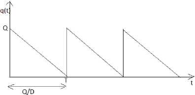
Fig 1.1. Development of inventory level over time

By solving the equation (3.1), we have q(t)=Q-Dt, for

0 < t < T (3.2)

And on using the boundary condition q(T)=0, we have

Q=DT. (3.3)

Holding cost,

IV. G eneralized EOQ M odel with linear trend of

DEMAND

We now generalize our discussion by accepting the equation (3.1) as a differential equation of fractional order instead of the linear order. i.e we here consider that demand(D) varies in fractional order say a , here instantaneous inventory level

= — D for 0dt^a

= 0 otherwise.                          (4.1)

where D=at+b ; a, b are constants.

Then we have the equation (4.1) as d aq (t) z

= — ( at + b ) for 0

dt ^a

= 0, otherwisw

With the same initial and boundary condition as described in the previous problem in equation (3.1). i.e q(0)=Q and with q(T)=0.

Equation (4.2) can be rewritten as

^C D ^α q(t) = -(at+b) for 0≤t≤T                 (4.3)

= 0 otherwise.

Where ^C D ^α ≡ J ^{1 - α} D ¹ is the Caputo fractional

1 d derivative as described in (2.2.9) and D ≡     .

To solve the initial value problem of fractional order differential equation (4.3) we apply the Laplace transform method. So taking Laplace transform of the equation (4.3), we have £ {C0Dtα{q(t)}= -£ {at+b}

⇒ sαq(s) -sα-0-1q(0) =-a- b , s s2

q ( s ) being Laplace transform of q(t).

aT ³ bT ²

HC 1,1 (T) = C ₁(      +      )

Case2: For β =1, Holding cost is T

HC 1, α ( T ) = C 1 ∫ q α ( t ) dt 0

T

= C 1 ∫ ( Q

-

= C 1 [ QT -

_at α + 1

Γ ( α + 2) _aT α + 2

-

-

bt ^α

)dt

Γ ( α + 1)

_bT α + 1

(4.1.2)

Γ ( α + 3)

= C [ ^{α + 1}   aT ^{α + 2}

¹ Γ ( α + 3)

(using (4.5))

Γ ( α + 2) α

]

+

Γ ( α + 2)

_bT α + 1_]

Case3: For α =1, Holding cost of order β is

HC 1, β ( T ) = C 1 D ^{- β} q ( t )

(4.1.3)

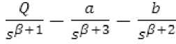
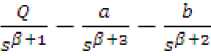
⇒ s ^α q ( s ) = Q s ^{α - 1} - ^a - ^b ₂

s s ² a b _s α + 2 ^- _s α + 1

⇒ q ( s ) = Q - s

Taking Laplace inversion of above equation we have,

q(t) = L ^{- 1}{ q ( s )} = Q -

_at α + 1

Γ ( α + 2)

bt ^α

Γ ( α + 1)

So the inventory level at any time t based on α ordered decreasing rate of demand is

_at α + 1 q _α ( t ) = Q -

Γ ( α + 2)

bt ^α

Γ ( α + 1)

for 0≤t≤T . (4.4)

on using the boundary condition q(T)=0 implies that

aT ^{α + 1}      bT ^α

Q=        +

Γ ( α + 2)   Γ ( α + 1)

(4.5)

A. Generalized Holding Cost:

Now the Holding cost of fractional order, say β i.e.

HC ( T ) = C D ^{- β} q ( t )                    (4.1.1)

Case1: For α =1 and β =1, Holding cost is

T

HC 1,1 (T)= C D ^{- 1} q ( t ) = C ∫ q ( t ) dt 0

T 2

= C 1 ∫ ( Q - ^at - bt ) dt 0 ²

Where q(t) = Q

-

aT ²

-

bT

at ²

Now { D ^{- β} q ( t ) }=^{      Q -

∴ D ^{- β} q ( t ) =Г-¹{

Qt ^β

β + 2 at ^{β +}

-

-

bt )}

} btβ+1

-

Γ ( β + 1)   Γ ( β + 3)   Γ ( β + 2)

∴ For t=T Holding cost

= ^C 1 [

QT ^β

_aT β + 2

_bT β + 1

-

-

Γ ( β + 1)   Γ ( β + 3)   Γ ( β + 2)

= C 1 [( ^aT + bT )

T ^β

aT ^{β + 2}

-

Γ ( β + 1)   Γ ( β + 3)

using (4.5) for α=1

β ( β + 3)

¹ 2 Γ ( β + 3)

aT ^{β + 2} + β

-

Γ ( β + 2)

]   (4.1.4)

bT ^{β + 1}

Γ ( β + 2)^]

bT ^{β + 1}} (4.1.5)

Case 4: For any α and β , Holding cost is HC  ( T )

= C 1 D ^{- β} q α ( t ) ,

Where,

α + 1 _at α + 1

q _α ( t ) = Q -

Γ ( α + 2)

=  { D ^{- β} [ Q

-

Q

-

bt ^α Γ ( α + 1) at ^{α + 1}

£ { D ^{- β} q α ( t ) }

bt ^α

-            ]}

Γ ( α + 2)   Γ ( α + 1)

a

b

,a+S+2 sa+S+i

^Л D e q a ( t )  -     {.__■__    ,.;-J-_:    ,.;-.•-.}

_   Qt ^в   _    at ^{a + в + 1} bt ^{a + в}

= Г ( в + 1)  H a + в + 2)   Г ( а + в + 1)

• — For t=T Holding cost

= C [ QT ^в -   aT ° ^{+ в + 1}    -    ^bT ° ^{+ в}   ] (4.1.6)

Г ( в + 1)   Г ( а + в + 2) Г ( а + в + 1)

= C [ , aT"+1      bTа , Tв       аТа+в+1        bTа+в]

Г ( а + 2)   Г ( а + 1) Г ( в + 1) Г ( а + в + 2)   Г ( а + в + 1)

Using (4.5)

C [ aT а+в+1{--------1---1}

=  ^1L       T( a + 2)Г( в +1)  Г( а + в + 2)    (4.1.7)

+ bTa+в {--------1---1}]

Г( а + 1)Г( в +1)  Г( а + в + 1)

F T= w d(w)                            (4.2.6)

G T ² = w d(w)

C

³ = w ₃ d(w)

(4.2.7)

(4.2.8)

T =

7 Г A

F

V G 1 7

'" 1 w 7

(4.2.9)

And G 2 C₃w ,3 — F ³ w 2 w₃ = 0

(4.2.10)

B. Generalized Total Average Cost

Total cost(TC) = Purchasing cost(PC) + Holding cost(HC) + Set up cost(SC).

Total Average Cost (TAC)= [Total Cost(TC)]

Case1 : For α=1 and β=1, Average Cost TAC* 1,1 (T*)

-³ [ UQ + HC_U(T ) + C 3 ]

1 2       32

aT          aT bT

= -^{[ U (}^- ^{+ bT} ) ⁺ C 1 ⁽^- ⁺ — ) ^{+ C} 3^]

= Ub + 1( aU + bC ) T + C^ T ² + C ³

2          ¹3         T

Now solve for w , w , w from three system of nonlinear equations (4.2.4), (4.2.5) and (4.2.10) and obtained the solutions as w ^* , w ^* and w ^* and then from the relation (4.1.16), we will able to obtain T ^* for which TAC 1,1 ( T ) is minimum. i.e we will able to obtain TAC ^* ( T ) as the minimum of TAC ( T ) in (4.2.1) and Q*(T) .

Case2 : For any а >0 and P =1,

Here,

TC _a ,1 (T )=UQ+ C [ ^LL aT a + ² +        bT “ + ¹] ^{+ C} 3

’              ¹ Г ( а + 3)         Г ( а + 2)

U [ ^aT—

Г ( а + 2)

= e₂t ^{a + 2}

bn ] + C [ - ^{а +1}- aT ^a + ²

Г ( а + 1)      Г ( а + 3)

+ FT ^{a + 1} + G₂T ^a

a

+--

Г ( а + 2)

bT ^a + i ] ⁺ C 3

+ C ³

T

(4.2.11)

C

= E + F T+ GT +                     (4.2.1)

Where E, =Ub, F. =   ( aU + bC ) &  G, = aC,

1                 1                                 11                1

Here the EOQ model is,

E

Where ²

n ^a + 1

= aC        F =

¹ Г а + 3) ,   ²

aU + bC _x a

Г ( а + 2) , &

C

Min TAC ( T ) = E + F T+ G T ² +   ³ ,  (4.2.2)

1,1                  1       1           1

subject to T ≥0,

(4.2.2) can be taken as a primal geometric programming problem with degree of difficulty (DD) =1.

Dual form of (4.2.2)

Max d(w) =

Subject to,

w 1

FL

V w 7

G'

w ₂

V w 2 7

( C 1 w

V w 7

(4.2.3)

w + w + w =1, (normalized condition)       (4.2.4)

w + 2 w - w =0, (orthogonal condition)       (4.2.5)

w 1 , w 2, w 3 ≥0.

Primal-dual relations are,

bU

² Г ( a + 1)

Then total average cost TAC  ( T )

= ¹ TC  ( T )

a ,1

= ET ^{a + 1} + FT ^a + GT ^{a — 1} + C ³

2  22

Here generalized EOQ model is,

^Min TAC „ ,1 ( T ) = E-T ^{a + 1} + FT ^a + GT ^{a — 1} + C ³ ,  ⁽4.2.¹²⁾

subject to T ≥0,

(4.2.12) can be taken as a primal geometric programming problem with degree of difficulty (DD) =2.

Dual form of (4.2.12)

f E.

Max d(w) = -^-

V ^w 1.

w 1

I    F ²

V W 2

w ₂

I f G 2

V ^w 3

w 3         w 4

I     C ³ I , (4.2.13)

¹ V w 4 7

Subject to, w + w + w + w =1, (normalized condition) (4.2.14)

W j ( a +1)+ a w ₂ +(a-1) w₃ - w ₄ =0, condition) (4.2.15)

(orthogonal

w 1 , w 2, w 3, w ₄ ≥0.

Primal-dual relations are,

E₂ T ^a ± 1 = W j d(w)

(4.2.16)

F₂T^a = w₂ d(w)

(4.2.17)

GT ^a 1 = w ₃ d(w)

(4.2.18)

= E₃ + FT + G₃T^{e + 1} + H₃T^e + ^3

Where, E, = bU , F =--- ,

,3           ,3       2, aC1^(P + 3)  p       bC1P

G^ = , &  H> =

³    2 Г ( в + 3)        3   Г ( в + 2)

So our model is min TAC1,p (T) = E3 + FT + G3Tp+1 + H3Te + C3

(4.2.24)

C у = w4 d ( w)

(4.2.19)

Using (4.2.16) and (4.2.17),(4.2.18) have,

(4.2.19) we

Subject to; T≥0

(4.2.24) can be taken as a primal geometric programming problem with degree of difficulty (DD) =2.

Dual form of (4.2.24)

T =	f F V E 2 J	I W[ V w 2 J	(4.2.20)
E 2 G 2 w 2		— F >2 W i W 3 = 0		(4.2.21)
And	a ± 1 G 2	w a W 4	— F2aC3 w 3 a + 1 = 0	(4.2.22)

f F )

Max d(w)= —

V W 1 J

w

f G 1

V ^W 2 J

w

H

V ^w 3 J

w ₃

f C 1

V ^W 4 J

w ₄

Subject to,

W ] + w₂ + w₃ + w ₄ =1 (normalized condition) (4.2.25)

Now solve for w , w , w , w from four system of non linear equations (4.2.14), (4.2.15) and (4.2.21) & (4.2.22) and obtained the solutions as w ^* , w ^* ,

**

w & w and then from the relation (4.2.20), we will able to obtain T ^* for which TAC ( T ) is minimum. i.e we will able to obtain TAC ^* ( T ) as the minimum of TAC ( T ) in (4.2.12) and Q*(T) .

Case3: For a =1 and for any P , we have the Holding cost ,

w₁ + ( P + 1) w₂ + e W ₃ - w₄ =0

(orthogonal condition)

the primal-dual relations are

FT = w d(w)

G T л ± 1 = w^ d(w),

HT ^p = w₃d ( w )

C

And у = W₄d ( w )

On using the above primal dual relation we get

T =

v

H 4 G

w

^W 3 J

(4.2.26)

(4.2.27)

HC_{V p} ( T ) = q{.

в ( в + 3) _Qв +2₊ в

2 Г ( в + 3)

Г ( в + 2)

bT ^e ± 1 }

G ₃ ^{1 P} H₃ w ^ w_Y — F₃w f w ₂ = 0

(4.2.28)

[from(4.1.5)]

Then Total cost

And G ₃ ² C₃w 2 w ₃ — F₃H ₃ ² w 2 w ₄ = 0

(4.2.29)

(TC) =UQ+ c { FF ± 31 aT e + 2 + ¹ 2 Г ( в + 3)

aT ²

Where Q= 2

/. Total average cost

---^в---bT ^{e + 1}} + ^C 3

Г ( в + 2)      '

TAC ( T )= ¹

1, ^e ’ t [ ^UQ+ C {

= -[ U( aT- + bT )

T 2

⁺ C { ^{e ( e} ± ³⁾ aT ' ± ² + 2Г( в + 3)

в ( £ ±31 aT « ± 2 +

P

2Г( в + 3)       Г( в + 2)

bT ^{6 + 1}}± c ₃ ]

^в    bT в ± 1 } + C 3 ]  (4.2.23)

Г( в + 2)     ^f

of TAC ( T ) in (4.2.24) and Q*(T) .

Case4: For any a >0 and any P >0, we have the Holding cost as

HC a,p (T ) =

C 1

Г(а + 2)Г( в +1)  Г(а + в + 2)

Г(а + 1)Г( в +1)  Г(а + в +1)

w 1 , w 2 , w 3, w , w ≥ 0.

Again the primal-dual variable relations are given by

ET ^{а - 1} = w , d(w)

[from(4.1.7)]

Then Total cost

ТС а , в (Т ) =UQ+

аТ ^{а + в + 1}{-

C 1

Г( а + 2)Г( в +1)  Г( а + в + 2)

+ C

+ ЬТ ^{а + в} {

Г( а + 1)Г( в +1)  Г( а + в +1)

Where Q is given in(4.5)

/. Total average cost is given by ТАС .в (T )G{UQ+

(4.2.30)

C 1

аТ ^{а + в + 1}

Г( а + 2)Г( в +1)  Г( а + в + 2)

^{+ C} 3 ^}

+ ЬТ ^{а + в} (

Г( а + 1)Г( в +1)  Г( а + в +1) _

- E₄T “ ^{— 1}

+ FT “ + GT “ ^{+ в} + HT “ ^{+ в — 1} + C ³

T

(say)

(4.2.31)

Where E =

, F =            ,

Г ( а + 1)   ⁴ Г ( а + 2)

—

Г(а + 2)Г(в +1)  Г(а + в + 2) J ,

H 4 = bC 1

—

Г(а + 1)Г( в +1)  Г(а + в +1)

So our model is min TIC,в (T) = E4T“-1 +

FT ^а + GT ^{а + в} + HT ^{а + в — 1} + ^3

subject to; T≥0

Now to minimize TAC ( T ) , we apply geometric programming method, and the degree of difficulty(DD) is=3.

Max d(w) =

' E ⁴

к ^w 1

I “]■ F 4

к W ₂

w

I  С G4

¹ к ^W 3

w ₃

I  -4

1 к w4

I w ⁴ С С 3

к W 5

w ₅

Subject to,

w_t + w ₂ + w ₃ + w ₄ + w ₅=1 (normalized condition)

(4.2.32)

( а -1) W j + а w₂

+ ( а + в ) w ₃ + ( а + в - 1) W 4 - W 5 =0 (orthogonal condition)

(4.2.33)

FT ^а - w ₂ d(w)

GT ^{а + в} = wd ( w )

H 4 T ^{а + в - 1} = w 4 d ( w )

³ = w d(w)

On using the above primal dual relation we get

T =

H 4 w ³

к G4 Jk w4 J

(4.2.34)

E₄G₄w₂w ₄ — P₄H₄w_xw₃ = 0            (4.2.35)

E ₄ ^{+ 1} w ₂ ^а w ₅ — F “ C₃w “ ^{+ 1} = 0             (4.2.36)

H 4 ^в W з^{в — 1} w 2 — F 4 G . w^3 = 0

(4.2.37)

Now solve for w , w , w , w , w from above five system of non-linear equations (4.2.32), (4.2.33) and (4.2.35) , (4.2.36) &(4.2.37) and obtained the solutions as *         *            ^* **

w , w , w , w , w and then from the relation (4.2.34), we will able to obtain T ^* for which TAC 4, в (T ) is minimum. i.e we will able to obtain tac 4 , в ( t *) as the minimum of TAC ( T ) in (4.2.31) and Q*(T)

V. C onclusion

In this paper, we have developed a classical EOQ model to a generalized EOQ model using the concept of fractional order differential calculus on the assumption that the demand to be a linearly increasing function of time and no shortage to be allowed. Although fractional calculus is much more complicated, still it has a potentiality to describe any other classical model to more general model precisely. Here it is shown that classical EOQ model is the particular case of generalized EOQ model. In future work, fractional differential calculus can be used to develop any other EOQ model in its more generalized form.