Graphical Programming Environment for Performing Physical Experiments

Published Online February 2020 in MECS DOI: 10.5815/ijmecs.2020.01.02

The evolution of science, in particular of engineering sciences, requires changes in teaching the introduction of interactive methods [1]. Interactive teaching strategies promote active learning teamwork involving students for achieving preset goals. The teacher becomes the transmitter of information organizer, facilitator, and mediator of learning activities. This way of teaching no longer centers on the teacher, but the student's learning process and facilitating skills development.

Using virtual laboratories [2] and modern methods based on computational technology [3,4,5] in the teaching activity to the student in engineering creates favorable conditions for obtaining useful skills in the workforce.

For physics applications requiring data acquisition, the activity requires some specialized resources and greater user experience. The block diagram of the pilot installation (Fig.1) comprises in general: PC (communication / display data input work order entry, etc.), software (generator software) acquisition board (the interface, the converter), the physical studied (information generator / physical signals), the sensors (signal transducers) program for receiving and processing the acquired signals, and PC (communication / display output data, output data storage, output work orders, etc.)

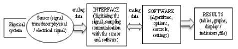
Fig. 1. The block diagram of the pilot installation

This paper presents, as a case study, the verification of the law of magnetic circuit in a simple circuit supplied with a DC voltage with a triaxial magnetic field sensor HMC5983 and data acquisition board MyRio 1900 from National Instruments. For the user interface it is used a Labview application . With law of the magnetic circuit is calculated the magnetic induction in the different systems of conductors and with the experimental instalation described above, the magnetic induction in these systems is measured.

LabVIEW is one of the first graphical programming language used in data acquisition applications with computers. With the data acquisition card, analog or digital data stream from the various transducers can be processed or analyzed [6,7,8,9,10,11,12,13].

Using LabVIEW for experimental physics provides many benefits such as the use of different types of sensors to track and measure variables during an experiment, the possibility of using systems of data acquisition for monitoring variables in computer applications, using virtual instrumentation [14,15].

• II.    Law of the Magnetic Circuit And Calculation Of The Magnetic Induction In The Different Systems Of Conductors

The law of the magnetic circuit [16,17], states that the magnetomotive voltage force along a closed contour Γ is equal to the electrical current conduction through any surface which rests on the contour plus the time variation of the flow electric through this area. (Fig. 2). To associate the elementary displacement vector dland the unit normal vector n dS = ndS it is used the drill rule. The default integral formula is:

^umm Γ ^{= i}S Γ

∂ ϕ _S +

∂ t

where u mm _r = J H • dl , i _S = JJ J • dS Γ           S Γ

Ф S _Г = JJ D • dS S Γ

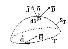
Fig. 2 Notations for law of the magnetic circuit

With the explanations from (2), the law may be presented in explicit integral form as:

J H l • dl = JJ J • dS + — JJ D • dS       (3)

Γ       S Γ      ^{∂ t} S Γ

The second term of the right member of the current intensity is called Hertzian.

If the environment is immobile, the derived from the right member enters under the integral as a partial derivative for a time of the electric induction. By turning the left-hand side of (3) with the formula of Stokes law is set as the local (in areas of continuity and smoothness)

∂ D rotH = J +

∂ t

If the medium is moving, as the curve Γ and surface S Γ is considered joint with the environment, thus derived from the right-entering into integration as substantial derived flow. Thus, as fully explained, the relation (4) is:

J H i • dl = jj J • dS ; + jj

Γ      SΓ

l d fD i f ⋅ dS dt

or the local form (4) becomes:

- -d rotH = J + dt or rotH = J +---+ldivD + rot(Dxv)(7)

∂ t

In the stationary case, the law of the magnetic circuit is known in the literature as Ampere's theorem [16,17]. If stationary case the law of the magnetic circuit, as an explicit whole becomes:

J Hl • dl = JJ I? • dS or J Hl • dl = I(8)

Γ     SΓ or J B? • dl = ц JJ "J • dS  J BB • dl = pI(9)

Γ      SΓ where I is the stationary conductive current intensity which passes through the surface which rests on the curve Γ and the magnetic permeability of the environment. If through the bounded area by the closed curve Γ pass more currents, it is made the algebraic sum of the current intensity. The intensity of the current which sense is given by the right end of the drill rotated in the direction of travel on the curve Γ is considered positive. From (6), when stationary, is obtained:

rotH = J               (10)

or rotB = pJ                (11)

• (8)    ÷ (11) is known in the literature as a mathematical form of Ampere's theorem.

It will be calculated is, using the law of the magnetic circuit, the induction of the magnetic field created by a linear conductor of finite length with the constant intensity current I - Fig. 3.

The physical model is shown in Fig. 3. To model the finite length of wire, as the current can not leave anything and can not disappear at the other end, it is considered at both ends by a time-varying electric charge q (t), and +q(t) to shape of the thread supply, such that:

I = - ^dq                 (12)

dt

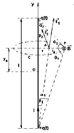
Fig. 3. The calculation of the induction magnetic field created by a finite length conductor passed by a current of constant intensity I

^ ⁽t) = 0 6 0 ^E y ^(r.^t) • rn- dr =

= q^(t)

d ^ dt

— I

______ ^{1/2 + y}0 ______

2 [(1/2 + У 0 )² + r 0 ]^{7 /} 2

—

¹ / ^{2 — y} 0

22(1/2 — y 0 )²

^{1/2 + y} 0 ^{1/2 — y} 0

1/2                     1/2

^22(1/2 + y a )" + 0 ]      ^{2(1/2 — y} 0 ^{) -} + r 0 ^J

Replacing in the law of magnetic circuit we will obtain:

1 ^— j(     f т , ⁸V )_ Ц 0 ¹

B • d1 = Un I I +--I =----- x

^{) c}             ( d t )     2

1/2 + y 0              1/2 — y 0

, ^{[ (1/} 2 ⁺ y 0^{)2 + r}0^{2 ] 1/2}   \^{l/2 —} y 0^{)2 + r}2 ^{] 1/}2

^ =

= U ⁰ — ( cos a i + cos a 2 ) = U °— ( sin d i + sin 0 2 )

The decrease in time of the tasks leads to the variation in time of the electric field produced by the task, namely at the onset of a slipstream, which means the time variation of the electric flux through the surface enclosed by the contour C, which contributes to the magnetic field, according to law magnetic circuit:

Solving the integral it is obtained:

B = Mo⁴ ( sin ^ i + sin ^ 2 ) ^{4 n r} 0

—*    —*

^B • dl = ц ₀ I 1

₊d ^ d t

The result is identically obtained also by using the Biot-Savart-Laplace theorem [16,17].

For 9 1 = 9 2 = n /2, it is obtained the case of infinite long wire (r 0 <

To determine the electric flux at a given time t through the surface bounded by the curve C, we determine the vertical component of the electric field created at a point a distance r from the wire:

B = ^{M 0} I-

2 m"0

E y (r,t) = E i_y (r,t) + E 2y (r,t) =

q(t)

^{4 n:}0

cos P i             cos в 2

⁽l / 2 + ^y 0 ) 2 ^{+ r} 2   ^{(l/2 — y}0^ 2 ^{+ r} 2

cos P ! = .  ^{1/2 +} y⁰ ^= cos P 2 =

V (1/2+y0 Y+r2

^{1/2 — y} 0     (15)

^{( 1} / ^{2 — y} 0 Y ^{+ r} 2

If we replace the previous relation we obtain:

E y (r,t) = ^ (t) 4®^

_____ ^{1/2 + y}0 ______ _____ ^{1 /2} - ^y 0

Г             9     9 3/2 + Г             9     9!? /.

^{(1/2 +} У0)" ⁺ r" J      (1/2 - ^y 0)" ⁺ r " J

The electrical flow through the bounded surface by the c curve is:

which can be obtained directly with Ampère's theorem.

It will be calculated the induction of the magnetic field in the center of Fig. 4, driven by a stationary electric current intensity I, both with the finite wire model and with the infinite wire model.

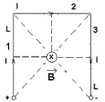
Fig. 4. The conductor framework which creates the magnetic field

We observe the three branches of the metal frame 1, 2 and 3. Branches 1 and 3 are of length L, and the length of branch 2 has l. The lines of the magnetic field created by a stationary linear electric current are concentric circles

with the axis of the conductor. The induction of the magnetic field is tangent to one field in each point line and has a constant value. The direction of the magnetic induction intensity is correlated with the sense current through the drill rule: rotating the drill to advance in the direction of flow through the conductor and the sense is the sense of induction rotating magnetic field or the direction of the magnetic field lines.

• A.    In the model using finite wire length

It is used the relationship (20) to calculate the contribution from each side after the superposition theorem is used to determine the total magnetic flux.

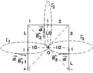
Fig. 6. The induction of the magnetic field in the center of a frame covered by a stationary electric current

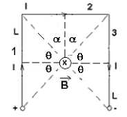
Fig. 5. Calculation of the induction magnetic field in the center of the wireframe model of finite length

The magnetic field lines passing through the center of the frame O, the field generated by the three branches of the frame are shown in fig. The inductions of the magnetic field have the same orientation at the point O, mainly they enter the plan of the figure and, according to the superposition theorem to calculate the total magnetic flux density B in O, are added together. So,

——  —  —

B = B i + B 2 + B 3 or B = B i + B 2 + B 3    (25)

Thus, following Fig. 4 or Fig.5, we will have:

—*     —*      —*       —*

B = B i + B 2 + B 3 or

To calculate each B₁,B₂,B₃ we apply Ampère’s theorem, explicit integral form:

B = B_t + B₂ + B₃ = ² ^ 0 ^I- ( 2 sin 0 )+^ ° L ( 2 sin a ) = 4 n l/2       ' 4~I. 2

Un I Г 2sin 0 sin a )

= ^-I+I

• п I lL

  
  

  which become:

  
  

—   —          —— f Bi ■ dl = UoI, f B2 ■ dl = UoI,(26)

Г 2

sin 0 =

L/2

V ( L/2 ) ² + ( l/2 ) ²

L

V L ²^ / ²

B i 2 n L = _{M o} i , B 2 2 n L = u o l , B 3 2 n l = M o I (27)

from where:

and l/2             l sin a =                   =                (23)

7 ( L/2 ) ² + ( l/ 2 ) ²    siL ² + 1 ²

We replace (23) in (22) and we will have:

B = — п •

и I Г 2L l )

7⁰    I —+ I

4L + 1² 1 ^{l L} '

Where ц _о=4 л- 1О^- 7 Н/т magnetic permeability of air or vacuum.

• B.    In the model using infinite wire length

We work with Amperè’s theorem ( see in Fig. 6).

Bi = B3 = M0^,B2 = ^I-(28)

пn

Thus

B = 2 Ml + Mo1 = mI Г 2 + 11

n l     n L     п ^ l L J

Next, the relations (24) and (29) are verified experimentally.

• III.    Describing the Experimental Installation

  The experimental installation, Fig. 7, comprises a rectangular frame with three branches, a battery, a digital multimeter, how GY-282 with the magnetic field high-resolution triaxial sensor HMC5983 [18], the plate data

  acquisition MyRio National Instruments 1900 [19], and a computer on which is installed a software acquisition board.

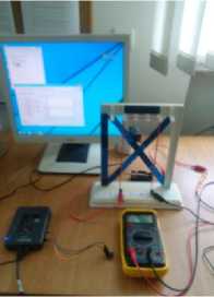
Fig. 7. Experimental components

Connecting the module GY-282 to the acquisition plate MyRio National Instruments is done according to Fig. 8.

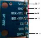
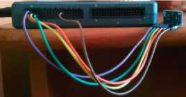
Fig. 8. Connecting the module GY-282 to the acquisition plate MyRio National Instruments (A connector)

The coordinate system of the magnetic field sensor is shown in Fig. 9.

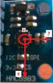
Fig. 9. The coordinate system of the magnetic field sensor

The interface application is carried out in Labview [20]:- Figs.10,11.

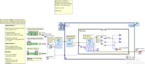
Fig.11. The application’s block diagram

• IV.    Results And Discutions

  With the frame size, L=23 cm and l=9 cm is calculated the magnetic induction in the center of the frame after the model of the finite wire B calculated,1 =1.7822 ⋅ 10^-5 T, with the relationship (24), and after the model of the infinite wire, B calculated,2 =2.1256 ⋅ 10^-5 T, with the relationship (29).The assembly of Fig. 3 is performed. Then the intensity of the electric current in frame is established at 2 A. It is executed the corresponding Labview VI application. The magnetic field sensor is placed in the vertical plan, in the center of the frame – Fig. 9. The geomagnetic field components of the magnetic induction are read – table 1.

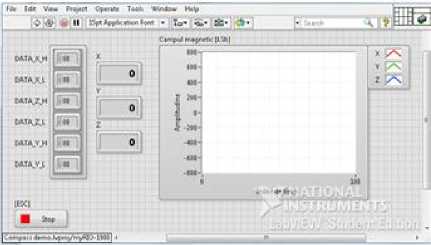
Fig. 10. The application’s front panel

To read the magnetic induction in the center of the frame the corresponding Labview application is run. The sensor is placed in the center of the frame with the Oz axis perpendicular to the frame – Fig. 9 and is read on the computer screen the magnetic field induction in LSB. It then subtracts the corresponding components of the geomagnetic field. The value of the LSB is then transformed into gauss, being given a corresponding configuration of the register B from the application (111, that is, FTT 230 LSB / Gauss) - Fig. 12. The value of B measured in gauss is then converted in tesla (1gauss = 10^-4T). The results are presented in table 2.

Table 1. The results of the measurements

The components of the geomagnetic field
Current number	B x (LSB)	B y (LSB)	B z (LSB)
1.	119	-145	93
2.	118	-147	92
3.	119	-153	94
Measurement results at current intensity 2A
1.	120	-149	52
2.	118	-150	51
3.	119	-145	54
Magnetic field in the center of the frame without geomagnetic field (average value) (LSB)
			-40.6666
Magnetic field in the center of the frame without geomagnetic field (average value) (T)
			1.7681 ⋅ 10-5
Magnetic field calculated with finite wire model (T)			1.7822 ⋅ 10-5
Magnetic field calculated with finite wire model (T)			2.1256 ⋅ 10-5

"11" is reserved

Configuration Register В

GN: Gain configuration, LSb/Gauss 1370 (000), 1090 (001), 820 (010), 660 (Oil), 440 (100), 390 (101), 330 (110), and 230 (111)

|GN[2:0]|

|ЙЙЙИИИИ|Д ]Щ гая

| M о de Register fC R), Add re s ;

Fig. 12. Configuration of the B register

From Table 2 is seen a very good agreement between the calculated value with finite wire model and the measured value.

• V.    Conclusions

Graphic programming environment removes the need to know a programming language. Instead of describing the calculation algorithm as a set of instructions in text format, a graphical programming environment the algorithm is described by drawing it as a logical scheme (block chart). The way in which the algorithm described is thus more intuitive and the program can be realized much easier especially for beginners.

In the case of the study experiment, is verified the law of the magnetic circuit using the GY-282 module with a triaxial magnetic field sensor HMC5983. This high-resolution sensor allows experimentation at low-intensity current being designed to measure the magnitude of magnetic fields, from milli-gauss to 8 gauss.

Such a working method for experimentation allows students to understand both the physical experiment and communication module of the pilot installation with the computer.