Graphical Representation of Optimal Time for a Step-Stress Accelerated Life Test Design Using Frechet Distribution

Published Online November 2014 in MECS DOI: 10.5815/ijitcs.2014.12.10

A more generalized case is used in step stress for the fulfillment of all the applications. Frechet distribution is important for modeling the statistical behavior of materials for a variety of engineering applications. It handles sensitive circuits very easily and is also used for opto electronic device such as solar cell, photo diodes, phototransistor, light emitting devices etc.

Due to continuous improvement in the technology, the products today have become more and more reliable with more life. It might take a long time, maybe several years, for a product to fail, which makes it difficult and even impossible to obtain the failure information under usage condition for such highly reliable products. So to get the information about the lifetime, a sample of these products is subjected to more severe operating conditions than normal ones to obtain its failure mode. This type of testing is called the accelerated life testing (ALT), where the products are put under higher than usual stresses to get more failure data in short time. The basic goal of ALT is to produce high quality product at low cost and less time .

The stress can be applied in different ways. Commonly used methods are constant stress, progressive stress and step stress:

• •    Constant-stress ALT : In this type, stress is kept at a constant level throughout the life of test products.

Some of the important early works in constant-stress test can be found in Kelpinski and Nelson [1], Nelson and Meeker [2].

• •    Progressive-stress ALT : In this type, stress applied to a test product is continuously increasing with time. See, Balakrishnana and Han [3].

• •    Step- stress accelerated life testing (SSALT) : In this stresses are increased in stepwise manner i.e. firstly the product is subjected to a specified constant stress S 1 , for a specified length of time. If it does not fail, it is subjected to a higher stress level S 2 until it fails. Since higher stresses are used for better result, so accelerated testing must be approached with caution to avoid introducing failure modes that will not be encountered in normal use.

For more Information about ALTs one can consult Nelson [4]. He was the first to propose the simple stepstress scheme, with the cumulative exposure model. Many studies regarding SSALT planning have been performed based on the CE Model, see Xiong [5], Watkins [6], Zhao and Elsayed [7], Balakrishnan el al. [8], Yeo and Tang [9]. Miller and Nelson [10] obtained the optimum simple step-stress accelerated life test plans for the case where the test units have exponentially distributed life times. Bai and others [11] extended the results of Miller and Nelson [10] to the case of censoring. Khamis-Higgins [12] introduced the step stress scheme for weibull distribution using K-H model. Ali and Ammar [13] proposed Optimal Design of Step-Stress Life Test with Progressively type-II Censored Exponential Data. Tang et al. [14] have used a linear cumulative exposure model to analyze data from a SSALT using 3-parameter Weibull distribution. Bhattacharyya and Soejoeti[15] developed a tampered failure-rate model. Bhattacharyya [16] also derived an approach using a Gaussian stochastic process which was later modified and extended by Doksum and Hoyland[17].

The cumulative exposure model defined by Nelson [4] for simple step-stress testing with low stress S 1 and high stress S 2 :

F(t ) =

F (t).F2 (t - T + <)

0 < t < tT < t < M

^Gi (t) = exp

; j = 1,2

where:

F i (t) the cumulative distribution function(c.d.f.) of the failure time at stress S i , τ is the time to change stress and τ' is the solution of F 1 (τ) = F 2 (τ').

On solving for τ' we get:

From (1) the PDF can be obtained by

g , (t) = -dG i (t) dt

Hence PDF is given by:

The Reliability function of Frechet distribution is:

81^(t )

where,

t — t + 9 2 t)

9 i ^J

0 <  t <  t

T <  t < M

V

R(t) = 1 - exp

\

t, a , 9 >  0

The remainder of this paper is organized as follows: In Section 2 we provide the simple conditions and assumptions on which whole paper is based. Next Section 3 presents the maximum likelihood estimators (MLEs) of model as well as Fisher Information matrix. Along with this variance-covariance matrix is also discussed. Section 4 gives the confidence interval details followed by calculation of optimal time with the help of graph in section 5. Section 6 explains the simulation studies for illustrating the theoretical results. Finally, conclusions are included in Section 7.

Notation:

K-H   Khamis-Higgins

PDF    Probability density function

MLE  Maximum Likelihood estimator

AV    Asymptotic variance

MSE   Mean square error

CI      Confidence Interval

N    total sample size ni    number of units failed at stress level i, i=1,2

• S 0     design stress

• S 1     low stress

• S 2     high stress

α    shape parameter

θ    scale parameter

β 0 , β 1 parameters of log linear relationship

τ     time to change the stress

Fi(t)  cumulative distribution function t1,j    observed failure times at low stress; j=1,…..n1

t_2, j     observed failure times at low stress; j=1,…..n₂

τ*      Optimal time

II. T he M odel and A ssumptions

The Cumulative Exposure model of a test product under simple stress test is given by:

G1 (t)

G(t ) =

L f.     9,G 1 t — t+t

2 V        9i

0 < t < tt < t < M

where,

g i^(t) = exp

V

—a

fl)

Ы, t, 9 i >  0

V⁹ i 7

The cumulative distribution function of the time to failure of a test unit under simple step-stress test follows the K-H model.

The K-H model for (1) is given by:

F(t M

0 <  t <  t

T <  t < M

a9 1 ^a t^{—a— 1}

a9 ^a t^{—a— 1}

exp<

0 < t <  t

T < t <  m

where log(θ i )=β 0 +β 1 S i , i=1, 2

Basic assumptions are:

• 1.    Under any stress the life time of test unit follows a frechet distribution with known shape parameter (α).

• 2.    Testing is done at two stresses S 1 and S 2 , with S 1 < S 2 .

• 3.    A random sample of n identical products is placed on a life test. First all test units are placed on low stress S 1 and run until time τ and then it is placed at higher stress S₂ until all units fail.

• 4.    The scale parameter θ_i at stress level i, i=1, 2 is a log-linear function of stress i.e. log(θ_i)=β₀+β₁S_i, where, β₀ and β 1 <0 are unknown parameters which is estimated by the data.

• 5.    The lifetime of test units are independent and identically distributed.

III. E stimation P rocess

A. Maximum Likelihood estimates

Let t ij , , i=1,2, j=1,2,….n i be the observed failure test of a unit j under the stress level i, where n 1 denotes the

number of units failed at stress S 1 and n 2 denotes the number of units failed at stress S ₂ respectively.

The likelihood function is given by-

—

52 log l 52 log l

WP 1

-V-P

ni г          1      n2

L^, e ₂;t) = П [ f i (t ij ) J + П   f 2 (т² Т + t₂ j —т )

Н               ■ ^{1        e} i

The log likelihood of the likelihood function is given by:

n1

logl = ?

[ f i (t i. ) ] + ?   f 2 ( p

■ ^{1             e} 1

^{т +} t 2j ^{— т )}

n1

logl =?

/ x —a

I t1i I loga + alog(e1) - (a + 1)log(ty) -1 I le1)

n2

+ ?

[ log a + a log e ₂ — ( a + 1) log(t ₂ . ) ]

n2

— ?

\ —a / x — a

1211  +1-^1

ej (ej

A^—a т I

—

e 2

The maximum likelihood estimates for β ₀ and β ₁ obtained by solving:

d logl 5p 0

n 1

= ? [ a + a t_1j

—<

- ^a e a ( P 0 +P 1 S 1 ) ]    +

be

d logl "dpT

= ? a2 S,t^e" (P+PS) j=1

n ₂

+ У S₂a ² 1₂^a * e^{a ( P} 0 ^{+ P} 1 ^{S 2 )}

22j j=1

+ Па a T

— I

a e a ( P 0 + P 1 S 1 ) S

— n2 a 2t-aSea(P0+PS2)

n ₂

z j=1

a — a (12“

_{— T}^-“ ) _e “ ( P 0 + P 1 S 2 )

_— а т—“ e “ ( P 0 + P 1 S 1 )

= ? Z [ a S! ( 1 — t _lj “ e “ ^{< ₽ 0 +P 1 S 1 )} ) ] +

n ₂ ? j = 1

aS— — aS₂ ( t₂ " “ — t "^a ) e ^{a ( P} 0 ^{+ P 1 S} 2 ⁾

— a S, t ^ e' ^{( P + e} 1 ^S 1 ⁾

= 0

= 0

A

A

the MLEs P ₀ and P ₁   are obtained and hence the

A

A

e ₁ and e ₂ can be obtained.

B. Fisher Information Matrix

The expected Fisher information matrix is obtained by taking the negative of the expected value of the second and mixed partial derivative of logl with respect to β 0 and β 1 which is given as follows:

E

—

I = n

E

—

d ² logl 5P 0 d ² logl dp 0 dp 1

E

E

—

d ² log l P

n ₁

—

—

d ² logl 5P 1 dp 0 d ² logl dp 2

n ₂

= ? a² 1 ^— “ e ^{a ( P} 0 ⁺ A S ⁰ + ? a² 1 ₂ ^— ; e “ ^{( P} 0 ^{+ P} S 2 ⁾

+ n₂ a 2 т " e ^{: ( P + №)}

—

n a ²t - “ e “ ^{( P} 0 ^{+ P S} 2 ⁾

d2 log l 5P12

E

E

E

—

—

? a2 S2te(в0+ j=1

n ₂

+ Xsa2 4"X(p0+ P S2) 22j j=1

,      2 a a ( P + P S )_c2

+ n2 ct t e (P0 P1 1) Sj

— n₂ a ² t "“S² e^{a ( p} 0 ^{+ P 1 S 2 )}

d ² log l ep 0

d ² log l d P d P .

—

d ² log l дв 1

where,

F = a ² exp

G = a ² < 1

exp

—

—

—

т

T 1

H = a²1 —

Ie 1

I = a²1 — (e 2

= A = F + G + H — I

= E

—

d ² log l

WP 1

= B

>

= FS, + GS2 + HS, — IS2

= C = FS ² + GS ₂² + HS ² — IS²

-a

-a

т

T 1

-a

т

T 1

-a

exp

—a

—a

т

T 1

+ 1

-a

+ 1 exp

—

-a

—

т

T 1

>

т

e ₂

The expected Fisher information matrix is given by:

I = n

AB

BC

The Variance and Covariance Matrix for MLE ( в 0 , (3 1 ) is defined as the inverse matrix of the Fisher’s information matrix:

X

n    C - B

AC - B 2 - B A

Elements A, B and C are given in (9).

When the exact mathematical expressions for the expectation is difficult to find then it can be approximated to the negative of the second and mixed partial derivative of log l with respect to P ₀ and 3 1 evaluated at MLE. It is known as observed Fisher information matrix, given by:

S =

_ d2l dp0 d 2l dP1dpo

d2l dp0dp1

d ² l

--- dP1 JPo =P0,P1 =P1

Elements of above matrix are given by (6), (7) and (8).

IV. C onfidence I nterval

The most common method to set confidence bounds for the parameters is to use asymptotic normal distribution of maximum likelihood estimators, see Vander Wiel and Meeker [18]. An estimate of a population parameter may be expressed in two ways:

• •    Point estimate: A point estimate of a population parameter is a single value of a statistic.

• •    Interval estimate: An interval within which the value of a parameter of a population has a probability of occurring.

In most cases, Statisticians use confidence interval to express the precision and uncertainty as they convey additional information than point estimate. For accurate construction of confidence intervals, the variance of the MLE is needed. So in order to construct the confidence intervals for parameters, we will use the asymptotic normality of the maximum likelihood estimates.

It is known that:

.0    0.            ..,     , .

(p o,Pi)~N((Po,Pi), X where, p0andp1 is the MLE of P0 and P1 respectively and X is the expected Fisher information matrix.

So Confidence Interval for population parameter P ₀ is given by:

P(L p o

o <  U p o ) = 5

where (L _Po

₀ < U_Po) is called two-sided 5100% confidence interval for в₀. L_Po and U p_o are the lower and upper confidence limits for β 0 . Therefore, the two sided approximate 5100% confidence limits for P ₀ and P ₁ are given respectively as follows:

_         0           .0 .               0           .0 .

Lp₀ =^p 0 ^{- /П}Ф 0 ) ^U p₀ =^p 0 + z ^ ( ^p 0 )

_         О           .0 .               О           .0 .

Lp_t =^p 1 - z ^ ( ^p 1 ) UP; =^p 1 ² z ^ ( ^p 1 )

V. O ptimization C riteria

An optimal test plan determines the type of stresses to be applied, level of each stress involved, methods used for stress application, minimum number of failures allocated at each stress level, optimum test duration by formulating the problem to minimize the AV of the MLE of a given 100 p ^th percentile at design stress.

The log of the 100 p ^th percentile of the lifetime t p (S 0 ) at the design stress S 0 is given by

V (S o ) = log(t p (S o )) =p о +P 1 S 0 + log( 9 i (logp) ^a )

The main purpose of this section is to explore the choice of τ in step stress accelerated life test which is obtained by minimizing AV of the MLE of a given 100 p ^th percentile at design stress S 0 . The AV is given by:

AV ( y > ( S o )) = log( t p ( S o ))

= AV ( в + в S о + log ^ Qog p ) " ^a )) ⁽¹²⁾

= ki к '= к X к'

where ,

Гау? (S o ) dy? (S o )"

K = —^--^—

L dpо    ap1 J and I-1 is the inverse of the expected fisher information matrix given in section 2.

So (9) becomes:

.       n(C - 2BS_n + AS 2 )

AV(t ? (S o )) = -(-------- ⁰₂   ⁰ )                      ⁽¹ 3)

AC - B ²

The optimum test plan for products having inverse Weibull lifetime distribution is to find the optimal time such that the AV(i? (S_o)) is minimized. The minimization of asymptotic variance over τ can be achieved by solving the following equation:

AV( ? (S o )) = 0

дт

The optimal time τ ^* is obtained by minimizing (13) with the help of MATLAB.

VI. S imulation S tudy

The main objective of this section is to illustrate how one can utilize the theoretical results discussed in the paper. In this we want to study the properties of parameter estimate and the respective confidence interval of parameters. We will also determine the optimal time which is obtained by minimizing the AV. So for the accomplishment of this task numerical example is presented.

Example:

Existing algorithms used in R and MATLAB to minimize the multivariable function is unable to calculate the minimum value of the above mentioned (13). So the value of stresses (S0, S1, S2), α, β0, β1 and τ cannot be found. Hence for minimizing the above equation following program is used.

For n=100, α=0.9(Shape parameter)

for(β 1 =1; β 1 <=10; β 1 = β 1 +0.05 )

for(β 0 =0.05; β 0 <=10; β 0 = β 1 +0.04 )

for(S 2 =1; S 2 <=10; S 2 = S 2 +0.05 )

for(S 1 =0.5; S 1 <=10; S 1 = S 1 +0.02 )

for(S 0 =0.8; S 0 <=10; S 0 = S 0 +0.1 )

for τ =0; τ <=100; τ = τ +0.1 )

Plot(AV( v (S o )))

By running the above pseudo code on MATLAB we find various plots between AV and τ for different value of parameters in given range. Among these plots, only one plot contains the minimum value of asymptotic variance for which the variables are τ^*=2.7, S 0 =1, S 1 =2.5, S 2 =3.5, β 0 =0.9 and β 1 =1.5. And this plot is shown as follows:

Fig. 1.

The time corresponding to minimum value of AV is called optimal time which is shown in the plot by τ*.

The steps involved in simulation procedure for example below are described as follows:

• a)    We simulate n=n₁+n₂=100 observations from K-H

model (section(2)) through above mentioned values.

The following steps are followed:

• •    Generate a random sample of size n from U(0,1) and arrange them in ascending order such that following conditions are fulfilled for stress S 1 and S 2 respectively:

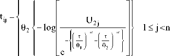
• •    Now tij are calculated as follows:

61[-log Uy)a

¹ <  ^j <  ⁿ1

• b)    For the selected values of parameter of β 0 & β 1 of, the MLEs P _oand Pj are calculated. Now calculate estimate of 0j and 0₂ by

θ i =exp(β 0 + β 1 S 1 )

• c)    The estimator’s performance is evaluated through MSE.

nS (m(ti)— mi)2

MSE = —------------ ; n- no. of observations. n

• d)    Calculate the observed and expected Fisherinformation Matrix then inverted to get the asymptotic variance and Covariance matrix of the estimators for different sample sizes.

• e)    The two sided confidence limit with confidence level δ=0.95 are constructed.

• f)    Finally, 95% confidence interval coverage is also

evaluated (approx and bootstrap).

—a

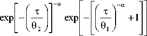
U_1j <  exp

—

and

< U2 j < «

The data in Table 1 includes 100 simulated observations from cumulative Frechet distribution (from (14)). Based on data the MLE of the model parameters β0 and β1 for τ*= 2.7, α = 3.19687 x 10-7, S1=2.5, S2=3.5, n1=73 and n2=27 obtained using maxNR option of R software are P0 = 11.204399 and P1 = -7.455094 and

P ₀ = 11.003689 and ft = -7.4026122

Table 1. Simple time-step stress with two stress variables simulated data

Stre -ss	Failure time
S 1 = 2.5	1.7409710 0.6210487 0.5063253 1.6659407 0.3442253 2.1263122 0.5201147 1.0874511 0.7994051 0.5688323 0.6176598 1.1802559 0.4691258 0.6387656 0.8261153 2.1902748 2.6739849 0.8353804 1.0384966 0.5183677 1.5472305 1.6485029 0.5249249 0.9808652 1.7549854 0.6157202 0.5165699 1.2507682 1.6814882 1.6929123 1.1389463 1.6159681 1.6042988 1.3683533 0.7943707 0.7561229 0.6310874 0.9460246 1.0763576 1.2558877 1.7383601 1.0066371 1.3683906 1.1006016 0.2761212 1.9954485 0.4924712 1.4892514 2.2951660 0.3277769 1.6643209 0.8057769 2.0116486 0.2454474 1.1508011 0.2118470 1.4312030 0.6142457 1.5209597 0.5894081 0.4044710 2.1414378 2.2078172 0.8950349 2.1160841 1.2699518 0.7810748 0.7114975 0.8962732 1.0496185 1.4962611 1.1451439 0.8203383
S 2 = 3.5	15.410737 4.785448   3.301290   17.781829 12.554463 4.6264830 3.364360   5.656238   5.281917   33.665982 2.7978460 3.096814   9.467507   4.972497  4.1984570 3.1623100 3.971346   2.726722   4.505802  2.7429090 3.5120310 22.67774  7.070494   4.215232  90.381085 12.277686 3.786421

Hence,

0 1 = 0.0005912 1 9 and 0₂ = 3.420086<10 ^-7

The Variance and Covariance Matrix for MLE

( (3 ₀, p 1 ) is defined as the inverse matrix of the Fisher’s information matrix:

The expected Fisher information matrix is:

I = 10^{- 11}<

1.021999 1.803055"

1.803055 1.875844

Sˆ

- 1

6.597070 -4.398047

-4.398047 4.398047

The asymptotic Fisher information matrix is:

0.4547474 0.4547474

0.4547474 0.6821210

Thus, the two-sided 95 per cent confidence intervals for (Po and P,), respectively, are

6.979256≤β 0 ≤15.42954, -10.90491≤ β 1 ≤-4.005279

Table 2. Parameter Estimation for the complete simulated sample for α=3.19687 x 10^-7, S 1 =2.5 and S 2 =3.5

n	P o P 1	MSE( P o) MSE( P i)	0 1 0 2	95% CI Coverage Approx   Bootstrap
20	11.066834	0.281725	0.000782362	0.93227	0.94828
	-7.4273632	0.986212	3.27154e-07	0.92871	0.93711
60	11.038761	0.075319	0.000653226	0.93582	0.93580
	-7.4408166	0.942323	3.077521e-07	0.93625	0.93781
80	11.009762	0.043211	0.0007352203	0.94631	0.94910
	-7.3076521	0.189263	3.325486e-07	0.94210	0.94730
100	11.003689	0.0043221	0.0005912119	0.95561	0.95291
	-7.4026122	0.182634	3.420086e-077	0.95681	0.95525
120	11.0026481	0.00442831	0.0003827629	0.95262	0.95891
	-7.5815421	0.0513122	1.7736314 e-07	0.95431	0.95790
200	11.0026534	0.0021831	0.0003286142	0.95831	0.95913
	-7.599231	0.0321322	1.6786132 e-07	0.95672	0.95885

Table 3. Parameter Estimation for the complete simulated sample for α=3.19687 x 10^-7, S 1 =2.9 and S 2 =3.6

n	- P o P 1	MSE( P o) MSE( P 1 )	0 1 0 2	95% CI Coverage Approx Bootstrap
20	11.068034	0.078391	0.0002583246	0.95423	0.95487
	-7.4378750	0.086243	1.608645e-08	0.95612	0.95675
60	11.061654	0.061833	0.000248978	0.96264	0.96968
	-7.4458631	0.083926	1.587544e-08	0.96710	0.96969
80	11.008321	0.0572453	0.000188765	0.96463	0.96721
	-7.5476521	0.0768253	9.964334e-09	0.96952	0.96967
100	11.003746	0.0527345	0.000178655	0.96742	0.96789
	-7.5626122	0.0582732	9.378544e-09	0.97315	0.97489
120	11.002146	0.0373531	0.000157543	0.97172	0.97257
	-7.5973442	0.0383645	8.178564e-09	0.97513	0.97845
200	11.0016534	0.019374	0.0001572322	0.97524	0.97598
	-7.5996511	0.001835	8.058956e-09	0.97972	0.97980

Table 4. Variation of optimal time (τ*) for α=0.9

	β 0 =0.9,β 1 =1.5	β 0 =1.1,β 1 =1.7	β 0 =2,β 1 =1.7
S 1 =2.5,S 2 =3.5	2.7	2.7	3.3
S 1 =2.5,S 2 =4.5	2.9	4.2	4.8
S 1 =4.5,S 2 =5.5	4.5	6.7	7.1
S 1 =5.5,S 2 =6.5	5.8	9.2	9.8
S 1 =6.5,S 2 =7.5	11.9	14.2	15.1

Table 5. Variation of optimal time (τ*) for different stress level

	n=100,α=0.9,β 0 =0.5,β 1 =1.5,S 0 =1.1
	* τ
S 1 =1.65,S 2 =5.06	2.7
S 1 =1.76,S 2 =5.06	2.7
S 1 =1.92,S 2 =4.18	2.7
S 1 =1.65,S 2 =4.62	2.8
S 1 =1.87,S 2 =4.62	2.8
S 1 =1.71,S 2 =4.5	2.7
S 1 =2.1,S 2 =4.48	2.8
S 1 =2.1,S 2 =4.76	2.7

• VII. C onclusion

Applications of Frechet distribution is more generalized for field of reliability. It handles sensitive circuits very easily and is also used for opto-electronic device such as solar cell, photo diodes, phototransistor, light emitting devices etc. The optimum plan is subjected to total number of test unit’s available, shape parameter (α), β 0 and β 1 . This approach of optimization is demonstrated by a numerical example, and the analysis shows that the initial value of parameters have little effect on optimal plans. Maximum likelihood estimators, Fisher information matrix (Expected and Observed) is also shown with confidence interval coverage of the estimators which is very high and stable. For some selected values of the parameters and stresses, we have shown in Fig. that as optimal time increases, the functional value (AV) also increases. Variation of optimal time for fixed shape parameter is also is also shown in table 4. From table 5 we conclude that Optimal time is stable when parameters are fixed while stresses lies between 0.6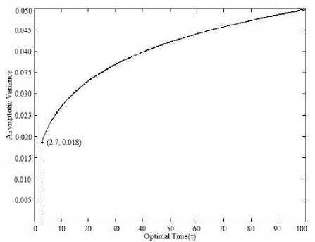1<2.7 and 1.022<3.6. Hence stress level has less impact on optimal time which suggests that the model is appropriate in the field of high reliability components.