Grass Fibrous Root Optimization Algorithm

Published Online June 2017 in MECS

Optimization is a mathematical technique to find the best solution of constrained or non-constrained problems. An optimization problem is how to find variables and parameters that minimize or maximize a function called the objective function. Many optimization problems have more than one local solution. Therefore, it is important to choose a good optimization method that globally looks to the search space to find the best solution without being trapped into local minima solution. Heuristics can be defined as approaches to find optimal or near optimal solutions in a rational computational time without a guaranteed to find an optimal value, while metaheuristics are a set of intelligent schemes that improve the efficiency of the heuristic procedures. Meta-heuristics can be classified according to the number of candidate solutions used at the same time. Trajectory methods are algorithms based on a single solution at any time and cover a local search based meta-heuristics, while population-based algorithms perform a search with many initial points in a parallel style. Meta-heuristic used in many scientific fields; such as neural network learning [1], and technical learning [2]. One of the most important population-based algorithms are the swarm intelligence algorithms. These algorithms were made of simple agents cooperating locally with each other depending on their environment, Each single element or particle follows one or numerous rules without any centralized structure for controlling its performance. Consequently, local and random interactions among the particles are directed to an intelligent global behavior. Many of these algorithms apply two approaches: global exploration and local exploitation, in which each particle improves its performance by co-operating, sharing information, and compete with other agents to survive. In spite of different nature inspiration sources of these algorithms, they have many similarities such as; initiate randomly, deal with uncertain, simultaneous computation, cooperation, competition, and iterative learning. Meta-heuristics algorithms dislike other exact mathematical methods, have no central control and if an individual fails, it does not affect the performance of the whole group. Therefore, they are more flexible and robust when acting on a complex, multimodal, and dynamic problems [3].

This paper proposes a novel meta-heuristic populationbased algorithm that solves complicated optimization problems. The inspiration of the proposed algorithm was the fibrous root system and reproduction process of general grass plants. In Grass Root Algorithm (GRA) the global search performed at each iteration, while the local search performed when the global search is in stack condition or it does not lead to more improvement in the objective function. In order to test the proposed metaheuristic GRA, seven standard test functions will be used. The obtained results will be compared with other nine well-known, and recently proposed algorithms which are Particle Swarm Optimization (PSO) [4], Differential Evolutionary algorithm (DEA)  [5],  Bee Colony

Optimization (BCO) [6], Cuckoo Search Algorithm (CSO) [7], Wind Driven Algorithm (WDA) [8], Stochastic Fractal Search (SFS) [9], Symbiotic Organisms Search (SOS) [10], Grey Wolf Optimizer (GWO) [11], and Novel Bat Algorithm (NBA) [12].

• II.    Related Works

Many meta-heuristic optimization algorithms have been proposed in the last few decades. These algorithms optimize an objective function to get the optimum solution using two individual mechanisms; global exploration and local exploitation. In 1995 Kennedy and Eberhart [4] propose an algorithm inspired by social behavior of bird flocking or fish schooling called PSO. It shares many similarities with evolutionary computation techniques. PSO algorithm initialized with a population of random candidate solutions and searches for best solution by updating generations. In 2005 Dervis Karaboga [6] proposed an algorithm motivated by the intelligent behavior of honey bees called Artificial Bee Colony (ABC). ABC algorithm uses only common control parameters such as colony size and maximum cycle number. It provides population-based search techniques in which foods positions are adapted by the artificial bees with time. Bee’s aim to explore the positions of food sources that have high nectar amount. In 2010 Z. Bayraktar and et al. [8] propose a novel WDO. It was a population-based iterative meta-heuristic optimization algorithm used for multi-dimensional and multi-modal problems. In WDO, small infinitesimally air parcels navigate over a solution search space follow Newton's second law of motion. WDO employs gravitation and Coriolis forces, provides extra degrees of freedom to fine tune the optimization.

This work proposes and implements a general grass root optimization algorithm GRA, comparing it with other meta-heuristic algorithms through using a variety of test function to evaluate the average mean absolute error, average number of effective iteration, and average effective processing time.

• III.    Grasses Development and Reproduction

There are three kinds of grasses fibrous root system which is; primary, secondary and hair roots. Primary roots are the first grown roots from the germinating seed. They provide the first few leafs with the required energy and minerals and stay active for a short period until the secondary roots become functional, then they die. Before the primary roots died the plant initiate new roots called secondary roots that develop at the same time new tillers and shoots. As energy is produced by developing leaves, some carbohydrates are partitioned to secondary roots for growth. These roots must compete with other neighbor roots to absorb water and minerals as they take over the function of the primary root. Hair roots are very small branches grow out of the epidermis of secondary roots. They absorb most of the water and minerals for the plant.

There are two major asexual reproduction methods in grasses; stolons which are stems creep along the ground, and rhizomes which are stems grow below the ground. Grasses use stolons and rhizomes to reach farther places and establish new grass culms [13]. Fig. 1 shows the grass asexual two reproduction methods.

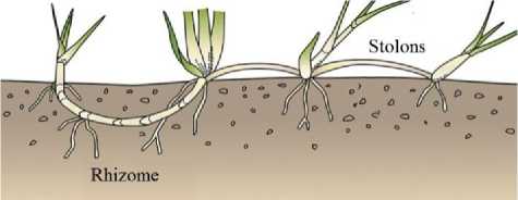
Fig.1. Grass two asexual reproduction methods.

• IV.    The Proposed Algorithm Govern Rules

Grass plants with stolons and rhizomes perform a global and local search to find better resources by reproduction of new plants and developing its own root system. Both the generated new grasses and roots are developed almost randomly. When a grass or root arrives at a place with more resources, the corresponding plant generates more secondary and hair roots, which makes the growth of the whole plant faster. If a grass plant has been trapped into local position it generates more new grasses by stolons initiated from the best-obtained grass and other grasses survived from the seeding process. On the other hand, new secondary roots with different deviation from the local minimum location will be generated by rhizomes. These secondary roots help plants reaching farther places and escaping from local solution. The rules that govern the grass model are illustrated as follows:

❖ Global search mechanism includes:

• •    Grass plants initiated randomly in the search space and only specified number of these plants survived according to the reached resources. The survived grasses generate a number of new plants deviated randomly from the original plants.

• •    The best grass obtained so far generates new grass plants using stolons. These  newly

generated grasses deviated from the best-obtained position with different search steps, usually greater than half of the maximum limit.

❖ Local search mechanism includes:

• •    The best grass obtained from the global search phase generates a random number of secondary roots using rhizomes. Each new generated secondary root contains hair roots equal to a problem dimensions.

• •    The secondary hair roots modify their length according to the step size vector.

• •    The best obtained secondary root in the local search phase generates new grass plants.

❖ The best-obtained grass grows faster than other and generates a larger number of deviated grasses and deviated secondary roots.

• V. Grass Roots algorithm Mathematical Model

As other meta-heuristic optimization algorithms, GRA starts with initial random population ( P ) in the search space domain of the problem. Each individual grass in the population represents a grass initiated by seeding process. When iteration ( iter ) begins, a new population ( NP ) will be generated. NP consists of the fittest obtained grass represented by GB = min( f ( P )), where f is the objective function, and D is the problem dimension, while the second element of NP is a number ( GN ) of grasses deviated from GB by stolons ( SD ). These stolons SD usually deviated from the original grass with step size usually less than the maximum limit of the upper bound ub , the last element of NP is new grasses equal to ( p– GN-1 ) deviated randomly from the survived initial grasses ( SG ), p represents the population size.

GN =

amse м p amse + minm Л 2

highest fitness initial population. The new population ( NP ) will be represented by (8).

NP = [ GB T , SD T , SG T J T         (8)

Grasses in NP will be bounded, evaluate their fitness and compared with the initial P . If the fittest new grass of NP is better than the old one of P then save the fittest new grass as the best solution. Otherwise, calculate the absolute rate of decrease in mse between the best obtained so far minimum mse ( bm ) shown in (9) and the current iteration minimum mse ( minm ) shown in (10). If the rate is less or equals a predefined tolerance value ( tol ) as in (11), then increase a global stack ( st g ) counter by one. When the st g reached its maximum value then move to the local search mechanism.

minm = mini =1,.,p (mse)

bm = min =1,.,iter (minmse)

minm-m.

------:------< tol , at j iteration(11)

amse

ps

= — ? mse_; ps ^T

no msei =       (dsj -yj )2               (3)

no 7 = 1

minm = min ( mse )                (4)

mse = ^ mse ₁,..., mse i , .., mse _ps J

Where GN is the number of generated new grass branches stolons SD deviated from GB . amse is the average of the Mean Square Error (MSE) values of all population mse , , are the desired and actual output value. Each new branch grass SD deviated from GB as in (6), while the survived deviated grasses SG is represented by (7).

SD = ones ( GN , 1 ) * GB + 2* max ( ub ) *...

( rand ( GN ,1 ) - 0.5 ) * GB

SG = GS + 2* max ( ub ) *...

( rand ( p ? GN - ,1 ) - 0.5 ) * ub

Where ones(c,1) represents ones column vector with c rows, and rand(c,1) is a random column vector with c rows ∈ [0,1]. Max(.) is an operator that finds the maximum element in a vector. GS is the ( p-GN-1 )

The local search mechanism consists of two individual loops; secondary roots, and hair roots loops. The secondary roots will be iterated by a random number usually less than problem dimension D . On the other hand, hair roots loops are equal to D. Therefore, each secondary root generated by the GB will represent a local candidate solution. Each single hair root modifies its location as in (12-15) for a repeated loops less than secondary roots number ( S ).

LB+1 = agb + GB^ + C 2* (£ - 0.5)

k=1,2,…,S and i=1,2,…,D.

D agb = 3 TRi(13)

i = 1

C = [0.02,0.02,0.02,0.2,0.2,2,2,2,2,15]

C 2 = C (1 + | 1^*10^)(15)

Where LB is the locally modified GB element by element, S is the number of secondary generated roots where (0 ≤S≤ D). C is the searching step size vector shown in (14), C2 is a random element of C chosen according to the percentage repetition of C elements as shown in (15). p and s are two random numbers £ [0,1]. If the evaluated locally LB minimum MSE lmin is less than bm, then save LB as GB. Otherwise, calculate the absolute rate of decrease in MSE as in (11). If the rate is less than tol then increase local stack counter (stl) by one, when stl reached its maximum predefined value then break hair root loop and begin new secondary root loop. After each completed iteration, check if the stopping condition (GError) is satisfied, then stop iteration. Otherwise, go to next iteration until reached the maxit then stop. Table 1 illustrates the general proposed algorithm pseudo code. The corresponding flowchart will be shown in Fig. 2.

• Table 1. GRA pseudo code

• 1:    Initialize maxit, p, D, lb , ub , GError, tol , st g , st l , C , GB ,

minm, bm , GN, f.

• 2:   Initialize random grass population P ∈ R^D

• 3:   Bound the initial population lb< Р < ub ub, lb ∈ R^D

• 4:   For i=1 : popsize // check for best fitness particle in the initial

population //

• 5:    F = f ( P ) // f is a predefined objective function //

• 6:   Calculate the mse ( i ) for F elements

• 7:   End For

• 8:   Sort the grass population ( P ) ascending according to mse

• 9:   For iter= 1 : maxit // global search starting //

• 10:  Evaluate C 2 according to (15)

• 11:  Generate the new population ( NP ) as in (8)

• 12:    Bound NP : lb< NP, NP, ub, lb ∈ R^D

• 13:     For i= 1 : p // check NP for the best fitness particle loop //

• 14:      F new = f( NP )

• 15:      Mse(i)= F new

• 16:     End For

• 17:   Minm=min( Mse ) // save minimum mean square error //

• 18:   Index the grass with the minm //index the position of the best

particle in the population//

• 19:   Evaluate GN deviated from as in (1). //GN is the number of

stolons or grass branches//

• 20:   Evaluate SO as in (6).

• 21:  Evaluate the GS from the ascending sorted P

• 22:   Evaluate SC as in (7).

• 23:  If Minm <  bm then

• 24:   bm=Minm

• 25:   GB =best indexed grass

• 26:   st g =0

• 27:   Else If (11) is true then

• 28:   increase st g by 1

• 29:   If st_g is at its maximum then

• 30:   st g =0 // Begin the local search //

• 31:      For q=1:S // secondary root loop//

• 32:       St l =0

• 33:        For j=1:D // hair root loop//

• 34:         LB = GB //initial LB//

• 35:        Evaluate LB as in (12)

• 36:          lmin = f( LB )

• 37:        If lmin then

• 38:         bm e =lmin

• 39:        GB = LB

• 40:          st l =0

• 41:        Else If (12) with lmin instead of minm is true then

• 42:         Increase st l by one

• 43:        Else

• 44:          st l =0

• 45:        End If

• 46:         If st_l is at its maximum then

• 47:        Break For

• 48:        End If

• 49:        End For (j loop)

• 50:      End For (q loop)

• 51:      End If

• 52:      End If

• 53:     If bm≤ GError then

• 54:      break For ( iter loop)

• 55:      End If

• 56:  End For ( iter loop)

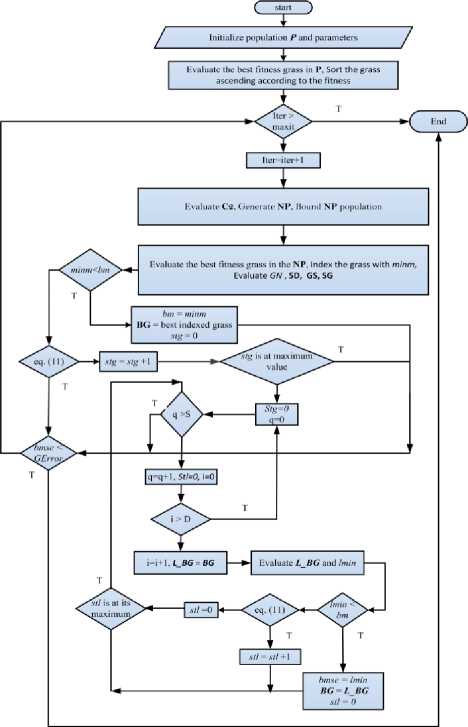
Fig.2. GRA flowchart.

• VI.    Test Functions Characteristics

Any new algorithm must have a validation for its performance by comparing it with other familiar algorithms over a good set of test functions. A common procedure in this field is to compare different algorithms on a large set of test functions. However, it is important to notice that the efficiency of an algorithm against others cannot be simply measured by means of problems that it solves, if the set of problems are too particular and without diverse properties. Therefore, in order to assess an algorithm, the kind of problems where it performs better than others must be classified, this is only possible if the test functions set is large enough to include an extensive variability of problems, such as multimodal, separable, scalable and multi-dimensional problems. The test functions used in this paper include multimodal functions which are functions with more than one local optimal, unimodal which have only a single optimum value that tests the ability of the proposed algorithm to escape local minima to a global one. The dimensionality of the search space and if the function is separable or not is another important issue related to the test functions.

• VII.    Experiment and Results

  In order to test the proposed algorithm performance, a comparison with other algorithms was carried out. DEA, PSO, BCO are well-known algorithms which have been widely used in optimization, while WDA, CSO, SOS, SFS, NBA, and GWO are more recently algorithms. These algorithms have been compared to GRA over different test functions. The variety of the used test functions and their characteristics give us an indication of the abilities of these algorithms. However, for the purpose of testing and implementation the compared algorithms MATLAB 2013 have been used on a core i3 2.4 GHZ CPU computer with 4GB ram. Each algorithm runs ten times for each test function to calculate the average Mean Absolute Error (MAE). All algorithms are set to have the same; p , maxit , and GError , which are equal to 10, 100, and 0 respectively. The proposed GRA algorithm tolerance tol were equal to 1e-2. Table 2 illustrates the obtained algorithms average MAE and the percentage successful of the ten complete iteration cycles for each algorithm. Table 2 uses 7 benchmark test functions to compare the performance of the proposed algorithm with other 9 metaheuristic algorithms.

However, the proposed algorithm has succeeded to optimize 85.71% of the test functions with 100% successful iteration cycles, as compared to 42.85% for SFS, 28.57% for SOS, 14.28% for NBA and WDA, and 0 % for GWO, DEA, BCO, CSO, and PSO. A small population size (10 particles) have been used to show the superior of the proposed algorithm over other tested algorithms. When increase the population size algorithms successful epochs rate will be increased. GRA algorithm succeeds to optimize Schwefel, and Michalewics test functions with 100% successful epochs and 50% for Dixon price, while other algorithms get 0% successful epochs for the same functions. Table 3 illustrates the effective average iterations number required by each algorithm to optimize each test function for the carried 10 cycles, while Table 4 illustrates the average effective processing time required to the effective average iteration number showed in Table 3. The shadowed blue cells in Tables 2,3, and 4 represent the succeeded algorithms to optimize the intended test functions. Therefore, the comparison (Bold marker) of the average processing time and average iteration number in Tables 3 and 4 will be restricted to these values only.

Table 2. Tested algorithms effective average AMAE.

Function	AMAE	BCO	CSO	DEA	GRA	GWO	NBA	PSO	SFS	SOS	WDO
Ackley [14]	avg.	3.48	0.256	3.73	5.15E-15	0.769	1.52E-03	3.82	8.88E-16	2.87E-09	0.739
	%	0%	70%	0%	100%	0%	100%	0%	100%	100%	70%
Rastrigin [15]	avg.	136	37.6	270	5.68E-15	45.5	69.6	328	0	0	29.7
	%	0%	0%	0%	100%	0%	0%	0%	100%	100%	0%
Schwefel [15]	avg.	5080	8550	9710	0.00112	7510	7200	7910	4080	5340	11000
	%	0%	0%	0%	100%	0%	0%	0%	0%	0%	0%
Zakharov [14]	avg.	61.1	445	746	1.16E-19	281	411	427	1.92E-69	1.76	8.16E-04
	%	0%	0%	0%	100%	0%	0%	0%	100%	20%	100%
Dixon price [14]	avg.	25.2	118	186	0.335	1.38	1.05	204	0.671	0.667	0.933
	%	0%	0%	0%	50%	0%	0%	0%	0%	0%	0%
Michalewics [15]	avg.	1.29	4.72	7.35	2.97E-02	3.79	5.46	5.83	0.797	2.53	5.84
	%	0%	0%	0%	100%	0%	0%	0%	0%	0%	0%
Shekel [14]	avg.	3.27	6.49	9.52	5.01E-03	4.13	5.41	4.9	0.875	3.47	5.41
	%	10%	0%	0%	100%	20%	0%	0%	70%	40%	0%

Table 3. Algorithms effective iterations number.

Fn	BCO	CSA	DEA	GRA	GWO	NBA	PSO	SFS	SOS	WDO
Ackley	100	100	100	4.3	100	75.8	100	11	35	100
Rastrigin	100	100	100	7.5	100	100	100	11.1	53.8	100
Schwefel	100	100	100	100	100	100	100	100	100	100
Zakharov	100	100	100	9.3	100	100	100	10.1	100	27
Dixon price	100	100	100	100	100	100	100	100	100	100
Michalewics	100	100	100	100	100	100	100	100	100	100
Shekel	100	100	100	100	100	100	100	100	100	100

Table 4. Algorithms effective processing time (sec).

Fn	BCO	CSA	DEA	GRA	GWO	NBA	PSO	SFS	SOS	WDO
Ackley	1.14	1.14	2.00	0.30	0.62	0.53	0.54	0.31	0.74	0.61
Rastrigin	0.74	0.81	1.22	0.19	0.45	0.59	0.43	0.26	0.97	0.49
Schwefel	0.77	0.87	1.23	5.64	0.37	0.55	0.43	1.95	1.44	0.38
Zakharov	0.75	0.87	1.40	0.37	0.52	0.70	0.50	0.31	1.82	0.34
Dixon price	0.78	0.92	1.43	5.15	0.38	0.50	0.36	1.73	1.34	0.40
Michalewics	0.87	1.64	1.90	1.16	0.65	1.30	1.50	2.00	1.53	0.78
Shekel	0.73	0.76	1.33	0.65	0.50	0.65	0.48	2.10	1.44	0.48

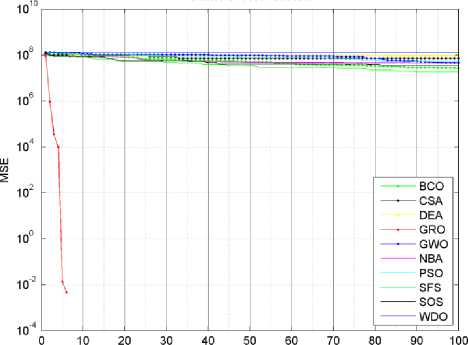
In Tables 3 and 4, we have seen that the proposed algorithm has gotten the lowest required effective iterations number for all functions succeeded to optimize. It also got the lowest required effective average processing time except for Zakharov test function. Actually, if we let algorithms complete the whole 100 iterations for each cycle. The proposed algorithm will require higher processing time than most of other tested algorithms, this is obviously clear in Dixon price test function. There are two reasons for this high processing time; firstly the proposed algorithm is more complicated than other tested algorithms, and the weakness in the trade off between the global exploration and local exploitation mechanisms. Figures (3-9) show the convergence curves for the tested algorithms, in which GRA converges faster than other algorithms. It also shows that GRA can reach an acceptable solution with fewer generations, fewer population, and fewer iterations as compared to other algorithms.

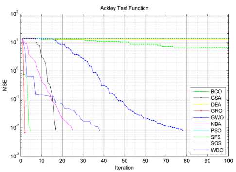
Fig.3. Ackley function algorithms convergence curves.

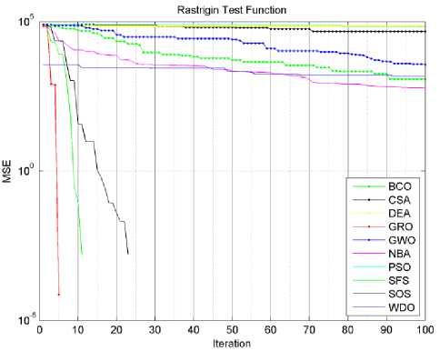
Fig.4.Rastrigin function algorithms convergence curves.

Schwefel Test Function

Iteration

Fig.5. Schwefel function algorithms convergence curves.

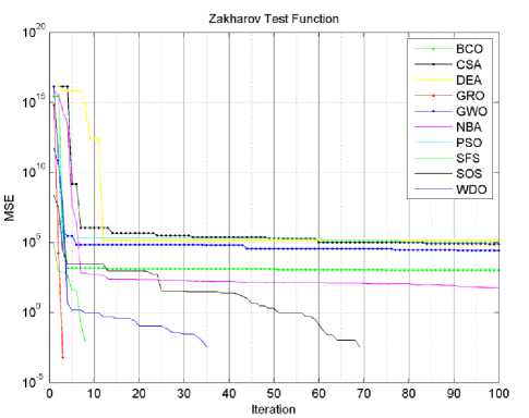
Fig.6. Zakharov function algorithms convergence curves.

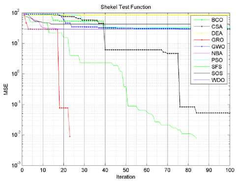
Fig.9. Shekel function algorithms convergence curves.

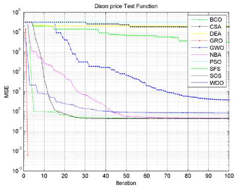
Fig.7. Dixon price function algorithms convergence curves.

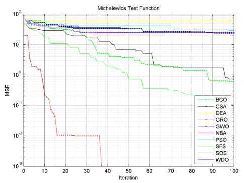
Fig.8. Michalewics function algorithms convergence curves.

• VIII.    Discussion

Any new optimization algorithm must have the ability to explore a specified search space (global search) and at the same time exploit the best-obtained solution (local search). Therefore, any optimization algorithm must equip with the two searching abilities to search new regions, especially around the previous best solution. However, a good tradeoff between the two features leads to a promising optimization algorithm.

• IX.    Conclusions

This paper proposes a new meta-heuristic optimization algorithm, inspired from the reproduction and root system of the general grass plants. GRA first search the problem using deviated from survived grasses, and reproduced grasses from the best grass for the global search, while secondary roots and hair roots are used for the local search. The performance of the proposed algorithm have been compared to familiar algorithms PSO, BCO, DEA, and other recently proposed algorithms SFS, SOS, NBA, GWO, CSO, WDA using seven test functions which have a variety of different characteristics. The obtained results showed that the proposed algorithm succeeded in optimizing test functions that cannot be optimized by other algorithms according to the chosen parameters and the search space limits, it also showed that GRA has faster convergence with a minimum number of iterations and generations than other compared algorithms.