Green’s Function Method in the Investigation of Dynamic Stability of a Fluid-Conveying Pipe

ВЕСТНИК ПНИПУ. МЕХАНИКА № 2, 2025PNRPU MECHANICS BULLETIN

Fluid conveying pipes represent a fundamental challenge in the field of fluid-structure interaction. The issue of dynamic stability of such structures has garnered significant attention in both scientific research and industry. Given that fluid-flowing pipes are integral components in numerous engineering facilities and serve as a primary means of transporting oil and gas, the stability of these pipes is of paramount importance. The loss of stability in a pipe can result in damages that have far-reaching consequences on the economy, the environment, and the well-being of the population.

M. P. Paidoussis is a distinguished scientist renowned for numerous publications in the field of fluid-structure interaction. His research, particularly focused on the interaction between flowing fluids and pipes, is extensively discussed in [1] and [2].

In their works [3] and [4], R. Gregory and M. P. Paidous-sis present numerical studies and results from experiments conducted on the dynamic stability of cantilevered pipes with flowing fluid.

In [5], an approach is presented for determining the circular frequencies and oscillations of a pipe conveying fluid. The transverse displacements of the pipe axis are also calculated. Additionally, [6] explores the vibrations of a pipe with a transverse linear elastic support.

A recent study on fluid-conveying pipes was conducted in [44]. Using the Euler-Bernoulli model, the authors investigated the stability of a pipe resting on a two-parameter elastic foundation, considering various boundary conditions. The Differential Transform Method was employed in the analysis. The results indicate that the elastic foundation has a stabilizing effect on the system, and increasing the foundation parameters leads to an increase in the system's critical velocity.

In a further recent investigation [45], the dynamic stability of a cantilevered pipe subjected to a lateral distributed load was analyzed. The Differential Quadrature Method was utilized in the analysis.

Ding and Ji [46] present a comprehensive review of the latest research in the field of vibration control for fluid-conveying pipes.

The broad applicability of nanoscale tubes across various scientific and industrial domains has sparked considerable research, as demonstrated in [9–16] and more recently in [47– 49]. To overcome the complexities and expenses of nanoscale experiments, fluid-structure interaction in carbon nanotubes is frequently studied using continuum elastic models, such as Euler and Timoshenko beam theories.

Curved pipes represent another area of fluid-structure interaction. Research in this area has been conducted in [33–38].

Other aspects of the problem of fluid-conveying pipe dynamic stability include pipes under thermal loads [26; 27], submerged pipe systems [19–21], and pipes made of viscoelastic materials [23].

Common methods for dynamic analysis of fluid-conveying pipes include the Finite Element Method (FEM), the Transfer Matrix Method (TMM) [39], and the Generalized

Differential Quadrature Method (GDQM). However, this paper proposes a different approach by suggesting the use of the Green’s Function Method to solve the stability problem. The objective is to demonstrate that this method can be competitive with the well-established techniques mentioned earlier in the dynamic stability investigations of fluid-conveying pipes.

The study in this paper focuses on a fluid-conveying pipe supported by linear elastic springs. The results obtained shed light on the relationship between the critical fluid velocity and the rigidity, as well as the number of elastic supports. The critical fluid velocity is the speed at which the flowing fluid leads to the loss of stability in the pipe.

The paper is structured as follows: first, we present the model of the pipe, including its static scheme, and the governing differential equation for eigen lateral vibrations. Second, we employ the Green’s function method to solve the problem, demonstrating the derivation of the frequency equation of the system. Conclusions about the system's stability can be drawn based on the roots of this equation. Finally, we present the results obtained from the numerical solution and summarize several key conclusions. To verify the results, they are compared to numerical results obtained using the Transverse Matrix Method for the same system. Furthermore, we offer our perspective on the key advantages and disadvantages of the Green’s function method compared to other methods for the dynamic investigation of pipe systems.

Problem formulation before deformation, remain plane and orthogonal to the deformed axis of the pipe;

• d)    Length of the pipe is significantly greater than the dimensions of the cross section;

• e)    The pipe is assumed axially inextensible;

• f)    The effects of rotary inertia are neglected;

• g)    The material of the pipe is linear elastic (The Hooke’s law is valid);

Each term in equation (1) has the following physical interpretation:

• a) Coriolis force:

  2 m _f V

  
  

  ^w . д t д x

  
  

b) Inertial force:

^{д 2} w

(mf+ mp )^T ■

c) Centripetal force (arising due to the acceleration of fluid through the deformed pipe):

- д ² w mV д? •

• a) The force in the j -th elastic support

w = K£ (x - xj) = 0.

j = 1

The pipe depicted in figure 1 is presented for analysis. It is hinged at it’s both ends and on intermediate linear elastic supports. The differential equation below describes the lateral vibration of the pipe.

д ⁴ w           д ² w        д ² w

EI + mr + m„    + 2 mV+ дx4 ( f p’дt2 f дtдx

+ mV ² ^ w + wYK ,8( x - x , ) = 0.

f   д x²      == j ⁽ j ’

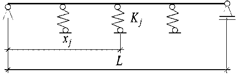
Fig. 1. Static scheme of the pipe

In equation (1), t is the time and x is the axial coordinate of a random cross-section of the pipe (Fig.1). w ( x , t ) denotes the function describing the transverse displacements of the pipe’s axis. The remaining system characteristics include the velocity of the conveyed fluid V , the bending stiffness of the pipe EI , the mass of the fluid per unit length of the pipe m_f , the mass of the pipe per unit length m_p and the rigidity of the linear intermediate supports K_j . δ is the Dirac delta function.

Equation (1) is valid under the following assumptions [1; 2; 8]:

• a)    Dissipation and damping effects are neglected;

• b)    Transported fluid is heavy, unviscous, and incompressible. This allows us to assume that the fluid velocity is uniform across the cross-section;

• c)    The Euler-Bernoulli hypothesis is valid. This implies that plane cross sections, orthogonal to the axis of the pipe

The dimensional equation (1) is converted into a non-dimensional form by introducing the following dimensionless parameters.

^ = x ; ^-

Lj

x

L

w y=L;

u = VL   '- ;

m в = —f—; mf + mp

t EI

^T =~vJ -------;

L m_f + m_p

Q = ю L²

EI mf + mp

KL ³ k = —, j _EI

where β is the mass ratio, u represents the dimensionless parameter associated with the fluid velocity, τ is the dimensionless parameter associated with the time, Q is the non-dimensional parameter of the pipe’s circular frequency and k j is the non-dimensional parameter of the rigidity of the elastic supports.

Following the mentioned transformation, equation (1) takes the following form:

д У 2 д y nr д y д y   n^ j

——z + u 7— +2 2 л/в u~— +^—г+ У/ ki ^(^ - §/ ) = 0-(3) д § ⁴    д § ²       дтд § д T ² J j

The solution of the differential equation (3) is sought in the form:

у ( §, т ) = w ( § ) e “' ,                         ⁽⁴⁾

where i is the imaginary unit.

By substituting (4) in (3) the following equation is derived:

W IV + u ² W¹ + 2^ Ui Q W -Q² W + W У k_J 8 ( § - § j ) = 0.(5) j = 1

The subsequent property of the Dirac delta function is employed [7]:

У ( § ) 8 ( § - § j ) = y ( § j ) 8 ( § - § j ) .            (6)

As a result, equation (5) obtains the following form:

W^IV + u ² Wⁿ + 2^ ui Q W¹ -Q ² W = - ]T k _j W ( ^ _j ) S ( ^- J (7) j = 1

The solution of equation (7) can be expressed in this manner:

W (§) = -ZkW(§,) G (§,§,), j=1

where G ( §; § j ) is the Green function, which satisfies the equation:

^-G + u2 ^-G + 2Jpui Q — -Q2G = 8(§-§/).

д §4 д §2 V д §            (

The Green’s function satisfies the same boundary conditions as W ( § ) . For the pipe in Fig. 1, these conditions are:

G ( 0; § j ) = G ( 1; § j ) = 0;

Gn (0;§j) = G" (1;§j) = 0.(10)

In equation (8) is substituted § = § i , i = 1,..., n , resulting in the following system of equations

W(§j) + t^W(§j) Gij= 0.(11)

j = 1

The system (11) has a nontrivial solution if:

k 1 G 11 + 1 k 1 G 21	k 2 G 12      • k 2 G 22 + 1	knG 1 n knG 2 n	= 0.	(12)
k 1 Gn 1	k 2 G n 2     •	■  kn G nn + 1

Equation (12) is the frequency equation of the system.

From it, the circular frequencies ω ₁,..., ω _n could be obtained.

The solution of equation (9) is as follows [8]:

^a M§ ^- J

G (§;§, ) = H (§ -§, )У   e+

⁽ “)     ^(S     ) ^ 4_а з + _2a a + ib

αi

α³ e ^{α i ξ}

+ w (0) У —3—i+ a 4a3 + 2a,a + ib αiii

2 £^a i ^

+ WI (0) У   , a'------- a 4a3 + 2a a + ib αi ii

+

^a i ^

+ [ ^W"" ( 0 ) + aW ( 0 ) + biW ( 0 ) ] У — - +

^L                              „ 4a. + 2a a + ib

αi

+ [ W I ( 0 ) + aW ( 0 ) ] У

α _i

α _ie ^{α i ξ}

4a³ + 2a i a + ib

In equation (13) a = u ², b = 2 ^u Q and c = Q ². H ( §;§ j ) is the Heaviside function and the coefficients a i , i = 1,....,4 are obtained as roots of the equation [8]:

z4 + az2 + ibz - c = 0.

The subsequent function is defined ^α i ^ξ

V( §) = У   ; e--------■

7^ 4a 3 + 2a i a + ib

Then, equation (15), for the pipe in figure 1, takes the form

G ( §; § j ) = H ( § - J v ( § - § j ) +

+ v '' ( § ) W¹ ( 0 ) + v ( § ) [ w¹¹¹ ( 0 ) + aW ' ( 0 ) ].

The values for W¹ ( 0 ) and W¹" ( 0 ) are obtained from the boundary conditions at the right end of the pipe.

W ( 1 ) = 0 ч G ( 1; § _J ) = 0;           (17)

W " ( 1 ) = 0 ч G " ( 1; § _J ) = 0.          (18)

Equations (17) and (18) are transformed in the form:

0 = v ( 1 - § j ) + v "' ( 1 ) W¹ ( 0 ) + + v ( 1 ) [ w'"' ( 0 ) + aW‘ ( 0 ) ] ;

0 = v "' ( 1 4 j ) + v "V ( 1 ) W " ( 0 ) + + v ¹¹¹ ( 1 ) [ W """ ( 0 ) + aW¹ ( 0 ) ] .

To obtain the critical velocity of the flowing fluid V_cr , an iteration procedure is applied. The velocity of the fluid is varied from 0 to the critical value V_cr , which corresponds to the zero value of the system’s first natural frequency.

Numerical results

eigenforms to 15 reduces the difference in the results of both methods to 3.3 %.

Numerical investigations were conducted for the fluidconveying pipe in Figure 1. Only the case with equal distances between the supports of the pipe has been considered. The material and geometric properties of the system are: modulus of elasticity of the material of the pipe E = 210 GPa , density of the pipe’s material

ρ = 7800 kg / m ³ . The outer and the inner radii of the pipe’s cross-section are R _out = 0.014 m and R _in = 0.012 m . Three different fluids with the following densities were considered: ρ = 1000 kg / m ³ ; ρ = 1100 kg / m ³ and ρ = 1200 kg / m ³ .

Figure 2 depicts the dependence of the critical velocity on the number of intermediate supports and their rigidity for a fluid with density ρ = 1000 kg / m ³ .

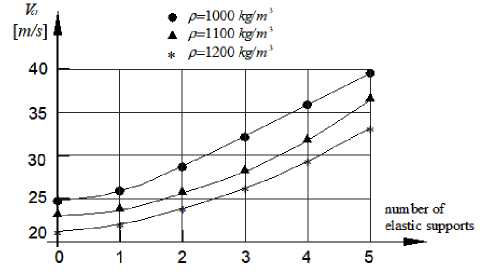
Fig. 4. Critical fluid velocity versus the number of intermediate supports for three different fluids with rigidity of the elastic supports K_j = 200 kN / m

Fig. 2. Critical fluid velocity versus the number of intermediate supports for a fluid with density ρ = 1000 kg / m ³

Figures 3 and 4 show the dependence of the critical fluid velocity on the number of intermediate supports for different fluid densities.

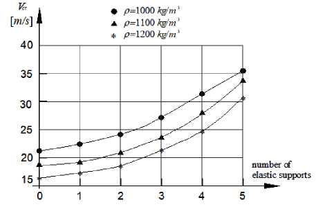
Fig. 3. Critical fluid velocity versus the number of intermediate supports for three different fluids with rigidity of the elastic supports K_j = 100 kN / m

A comparison has been made between the results obtained using the Green’s function method and the solution for the same system using the Transfer Matrix Method (TMM). When 10 eigenforms are used in the TMM solution, the results show an average difference of 5.4 % in the critical velocities obtained. As expected, increasing the number of

Conclusion

The utilization of the Green’s function method in this paper offers an alternative avenue for exploring the dynamic response of fluid-conveying pipes. The suggested approach can be regarded as a viable competitor to other established methods for dynamic investigation of fluid-conveying pipes, such as the Transferred Matrix Method, Generalized Differential Quadrature Method (GDQM) and Finite Element Method (FEM).

In the scientific literature, it has been shown that TTM and GDQM have a significant advantage over FEM. The FEM's application to pipelines with numerous spans results in a substantial increase in computational time, attributed to the expanding order of the system's property matrices. This contrasts sharply with the TMM, where the overall transfer matrix retains a fixed order, independent of the number of spans. The GDQM efficiently approximates derivatives in the pipe's lateral vibration equation by utilizing weighted sums of function values at discrete points, resulting in rapid convergence with a sparse grid.

Compared to the TMM, the Green’s function method has the advantage of not requiring the solution of the free vibration problem to determine eigenvalues and eigenfunctions, which are also essential in the classical Galerkin method.

Another significant advantage of the Green’s function method is that the accuracy of the solution does not depend on the number of finite elements (as in FEM) or the number of eigenforms used in the Galerkin method and TMM, as the method is regarded as equivalent to the exact analytical solution of equation (1) [8].

The suggested approach also has a significant drawback: it requires the use of a complex mathematical framework, which could make it less appealing for practical engineering applications.

Several major conclusions can be drawn regarding the numerical investigations presented in the article:

• 1.    The numerical results indicate that augmenting the number of intermediate supports enhances the system stability.

• 2.    Another notable observation is that boosting the rigidity of the elastic supports results in increased system stability.