Heterogeneous Energy Efficient Protocol for Enhancing the Lifetime in WSNs

Published Online September 2016 in MECS

Computer networks play a very important role in human life for exchange information/data using wired or wireless links. There have been new developments in network technologies and accordingly new network paradigms have been developed especially related to the wireless networks. The cellular telephones, mobile phones, laptops, and various types of personal digital assistants (PDAs), etc., are mainly used by hundreds of millions of people to wirelessly communicate. The wireless networks include ad-hoc networks, opportunistic networks, mesh networks, peer-to-peer networks, cellular networks, wireless local area network, and sensor networks. These types of networks do not require any fixed infrastructure and can be deployed easily in those areas where employing infrastructure is either not possible or difficult to lay down [1]. The wireless sensor networks (WSNs) are being increasingly used in hostile environments, such as high temperature and vibration, flood, volcano, landslide detection, glacier monitoring, chemical leakage detection in rivers, etc., where traditional network systems cannot be used. These applications of WSNs however have several restrictions, such as limited energy supply, limited computing power, and limited bandwidth of the wireless links connecting the sensor nodes.

Due to advancement in wireless technologies and their applicability, the wireless networks can be divided into two categories based on the architecture: infrastructurebased networks and infrastructure less networks. An infrastructure-based network has pre-constructed infrastructure; in other words, it has a fixed network structure, e.g., cellular networks and wireless local-area networks. It consists of the networked devices and the wireless access point or wireless router. Each device must be connected to the access point before having access to other computers in the network. An infrastructure less network has an arbitrary set of independent wireless devices and has no specific pre-defined role for each device, e.g., ad-hoc networks and wireless sensor networks. An ad-hoc network consists of nodes (computing/connecting devices) to communicate directly or indirectly to each other using the wireless transceivers without requiring a fixed infrastructure. The computing devices used in ad-hoc networks have relatively less computing power, but each of them in itself is a complete system. The wireless sensor networks are a new class of ad hoc networks that consists of low-power, small size with low cost as well as low complexity devices. These devices are called sensors. A wireless sensor network has many restrictions like memory, processing power and energy capacity in terms of their sensor nodes’ capabilities [2].

The wireless sensor networks (WSNs) contain hundreds or thousands of sensor nodes equipped with sensing, computing and communication abilities. Each node has the ability to sense the environment for an activity or object and can perform simple computations. A sensor node either communicates among its peers to collect the sensed data or sends (receives) the data to (from) a base station. A base station connects the sensor networks to another network. Designing protocols for sensor networks has to be energy aware in order to prolong the network lifetime, because the replacement of the embedded batteries in sensors is a very difficult process, once these have been installed. The WSNs should utilize their network energy in an efficient way so that they can monitor the environment for longer time. A sensor node is basically made of four components namely: sensing unit, processing unit, transceiver unit, and power unit. It may also have additional application-dependent components such as a location finding system, power generator, and mobilizer. The sensing units are usually composed of two sub-units as sensors and analog-to-digital converters (ADCs). The analog signals produced by a sensor based on the observed phenomenon are converted into digital signals by the ADC, and then fed into the processing unit. The processing unit, which is generally associated with a small storage unit, manages the events that make the sensor node collaborate with other nodes to carry out the assigned sensing tasks. A transceiver unit connects a node to network. One of the most important components of a sensor node is power unit, which may be supported by power scavenging units. Most of the sensor network routing techniques and sensing tasks require the knowledge of location with high accuracy. Thus, it is common that a sensor node has a location finding system. A mobilizer may sometimes be needed to move sensor nodes when required to carry out the assigned tasks [3].

The nodes in wireless networks can be deployed deterministically or randomly. The deterministic deployments are more preferable in applications where the deployment area is physically accessible. The examples include the line in sand for target tracking, city sense for urban monitoring, soil monitoring, etc., where the sensor nodes are placed manually at the selected locations. On the other hand, random deployment of sensor nodes are used when the deployment area is physically inaccessible, e.g., bird observation on Great Duck Island, Mines, etc. In such environments, the sensor nodes are dropped from an aircraft.

The most important issue in WSNs is related to longevity of the network, which is directly or indirectly influenced by the network energy. The efficient utilization of the network energy may be done by organizing the sensors into groups, called clusters. Each cluster has a master node, which is also called the cluster head and several sensor nodes as members of it. The cluster head usually performs the fusion and aggregation. This concept has resulted into the development of different protocols that helps in efficient utilization of the energy. In order to have longer lifetime, the network should have good amount of energy. The network energy can be increased by increasing the number of sensors in the monitoring area. Increasing the number of sensor nodes does increase the network energy, but the cost is quite high because deploying an extra sensor incurs the cost of the sensor, which is ten times more than the cost of the batteries. Therefore, it is more appropriate and economical to increase the network lifetime by deploying some sensors with high battery. The sensor networks with such characteristics, i.e., sensor node with different energy levels are termed as heterogeneous wireless sensor networks [4]. In this paper, we propose a 3-level heterogeneous network model for WSNs to prolonging the network lifetime. Our heterogeneous network model also helps to select cluster heads and their respective cluster members by using weighted election probability and threshold function.

The rest of the paper is organized as follows. Section 2 discusses the literature review. Section 3 discusses the proposed 3-level heterogeneity network model and clustering process of heterogeneous hybrid energy efficient protocol for 3-level heterogeneity network model are discussed. Section 4, experimental results are discussed and finally in section 5, the paper is concluded.

• II.    Literature Review

  The WSNs have attracted several researchers because of their potential applications and related challenges. They have several applications like military applications, environmental applications, health applications, scientific exploration, area monitoring and structural health monitoring, etc. At the same time, they have numerous challenges like simplicity, coverage, connectivity, scalability, robustness, fault-tolerance, security, efficient use of energy, deployment strategies, etc. One of the most important challenges is related to the enhancement of network lifetime so that it can observe the monitoring area for long time for the activities of objects. The network lifetime is essentially related to the efficient use of network energy. Accordingly, several approaches have been developed including various protocols. The very first protocol for increasing the lifetime in WSNs was discussed by Heinzelman et al. in 2000, which is known as low energy adaptive clustering hierarchy (LEACH) protocol [5]. It is one of the most accepted protocol based on clustering. In clustering, the sensors are divided into groups, each group is called as cluster. There is a master node in each cluster, called cluster head, that collects the data from its cluster members and sends that data directly or via some intermediate nodes to the base station. All sensors don’t send the data directly to the base station rather they send their data through cluster heads that is why it is called hierarchical protocol.

In LEACH, the cluster heads may not be dispersed uniformly in the entire region as they are selected randomly. Another problem in LEACH is that the number of cluster head nodes is not fixed due to stochastic selection. These problems have been addressed in LEACH-C and fixed LEACH [6], by dispersing the cluster heads all over the network so that it can produce better performance. In LEACH-C, the base station (BS) organizes the nodes and controls the network. In each round of LEACH-C, a node needs to send its residual energy and location information to BS. Based on the received information, the BS can uniformly distribute the cluster heads throughout the topology and adjusts the size of each cluster. The BS also adjusts the probability of selecting the cluster heads according to the nodes’ residual energy because the BS carries out energy intensive tasks like cluster formation and cluster head selection. In fixed-LEACH, the number of cluster heads is fixed. The sensor nodes choose their nearest node as cluster head where the number of supported nodes may be different for each cluster head. This leads to the uneven energy dissipation among the nodes. The LEACH has been modified by Lindsey and Raghavendra [7] and named as power efficient gathering in sensor information systems (PEGASIS) protocol. The PAGASIS protocol is nearly optimal in terms of energy cost for data gathering applications. The key idea in PEGASIS is to form a chain among the sensor nodes so that each node receives from and transmit to a closest neighbour node. The gathered data moves from node to node, gets fused, and, eventually, a designated node transmits it to the base station (BS). The nodes take turns in transmitting to the BS so that the average energy spent by each node per round is reduced. It has better network lifetime as compared to the LEACH because it uses only one node in a chain to transmit the data to the BS instead of multiple nodes. It, however, due to excessive delay, is not suitable for large networks.

The PEGASIS has been extended by forming the chain using binary structure so that the length traversed by a packet is reduced (balance the energy and delay cost) and this extended version is called as Hierarchical-PEGASIS [8]. Manjeshwar et al. discuss the threshold sensitive energy efficient sensor network (TEEN) protocol [9] based on hierarchical clustering. In this protocol, a cluster head broadcasts two thresholds to the nodes, which are called as hard and soft thresholds for sensed attributes. The hard threshold is the minimum possible value of an attribute to trigger a sensor node to switch on its transmitter and transmit to the cluster head. Thus, the hard threshold allows the nodes to transmit only when the sensed attribute is in the range of interest; thus reducing the number of transmissions significantly. The soft threshold further reduces the number of transmissions if there is a little or no change in the value of the sensed attribute. The TEEN is however not good for applications where the periodic reports are generated because some users may not get any data at all if the thresholds are not reached. Another problem with this protocol is that the base station never knows whether the un- reported nodes are dead or alive. The TEEN protocol has been extended in [10] and the resultant protocol is known as adaptive threshold sensitive energy efficient sensor network (APTEEN) protocol. This protocol is meant for capturing periodic data collections and time-critical events. It allows users to set threshold values and a count time interval. When the base station forms the clusters, the cluster heads broadcast the attributes, threshold values, and transmission schedule, to all nodes. The main drawbacks of the APTEEN protocol are overhead and complexity of forming the clusters. Ye et al. discus the energy efficient clustering scheme (EECS) protocol [11] that is used for periodical data gathering applications in WSNs. This protocol elects the nodes as cluster heads which have more residual energy through local radio communication while achieving good cluster head distribution. It however increases the requirement of the global knowledge about the distances between the cluster heads and the base station. Eshghi and Haghighat [12] discuss a technique which forms smaller clusters near the base station because the nodes nearer to the base station require to spend more energy than the farther nodes as the neighboring nodes of the base station have extra burden. Junping et al. discuss a time-based cluster-head selection algorithm for LEACH (TB-LEACH) [13], an improvement of the LEACH. In this algorithm, the competition for cluster heads does not depend on the random number as in the LEACH, but on the time interval. The sensor nodes which have the shortest time interval for each node win the competition and become the cluster heads while ensuring cluster partition balanced and uniform.

Younis et al. discuss hybrid energy efficient distributed (HEED) clustering protocol [14], an extension of the LEACH protocol, which uses two parameters for selecting the cluster heads. The primary parameter for cluster heads selection is the residual energy and the secondary parameter as degree of the node. The degree of a node and the number of nodes in its range, help in distributing the load among the cluster heads for load balancing. In this protocol, the clustering process is carried out in terms of iterations. In each iteration, the nodes not covered by any cluster head double their probabilities of becoming cluster head. It has low overhead in terms of processing cycles and message exchanged. This protocol does not assume any distribution of the nodes or location awareness. It also achieves fairly uniform cluster head distribution across the network and prolongs the network lifetime besides supporting the data aggregation. A variant of the HEED protocol, called integrated HEED (iHEED) by Younis et al. [15], discusses the integration of the data aggregation in multihop routing by considering the data aggregation operators such as AVG or MAX. The iHEED uses an energy consumption model to keep track of the battery consumption of the cluster heads and regular nodes. Another variant of HEED by Huang and Wu [16] discusses a constant time clustering mechanism that may be termed as an extended probabilistic algorithm for HEED protocol. In this algorithm, the nodes having high energy participate in cluster head election and the remaining large quantities of nodes are eliminated; thus, it requires fewer rounds for selecting the cluster heads.

For past few years, the WSNs have mainly focused on technologies based on the homogeneous WSNs in which all nodes have same system resources. Recently, the heterogeneous wireless sensor networks are becoming more and more popular. The researches [22-23] show that heterogeneous nodes can prolong the network lifetime and improve the network reliability without significantly increasing the cost. The heterogeneous nodes are more capable of providing data filtering, fusion and transport; but they are more expensive than the homogeneous nodes. A heterogeneous node may possess one or more types of heterogeneous resources, e.g., enhanced energy capacity or communication capability. Compared with the normal nodes, they may be configured with more powerful microprocessor or more memory or both. They may also communicate with the base station via high-bandwidth and long-distance network. There are mainly three types of resource heterogeneities in a sensor node that include computational, link, and energy heterogeneity. The computational heterogeneity refers to distinct ability of the node in terms of its computation. For example, some node may have more powerful microprocessor and some may have more memory and others may have both. The link heterogeneity refers to distinctness of capability among the links. For example, some links may have high bandwidth and others may provide longer distance network transceiving capability. The energy heterogeneity refers to different levels of energy among the sensor nodes. For example, some nodes may have more energy in comparison to other nodes. The computational and link heterogeneities implicitly depend on the energy heterogeneity as the nodes with computational and link heterogeneities consume more energy. Thus, the energy based heterogeneity can be considered as the most dominating heterogeneity in WSNs. If there is no energy heterogeneity, the computational and link heterogeneities will bring negative impact to the whole network, which can result in early shutting down the enire network. The deployment of heterogeneous nodes increases the network energy and hence the network lifetime.

There have been some works that discuss heterogeneous network models. Smaragdakis et al. discuss stable election protocol (SEP) [24], an extension of LEACH, that uses heterogeneity. It is the very first protocol, which talks about heterogeneity. In this protocol, a node becomes cluster head on the basis of weighted election probability, which uses a function of the remaining energy of the nodes to ensure uniform usage of node energy. The underlying network of the SEP considers two levels of heterogeneity, consisting two types of nodes, known as normal and advance nodes. The energy of the advanced node is higher than the normal nodes and their number is less than that of the normal nodes due to the increased cost factor. Let N be number of sensor nodes deployed in a monitoring area. Suppose, E 0 is the initial energy of a normal node and m is the fraction of the advanced nodes, which has a times more energy than a normal node. Then there are m * N advanced nodes equipped with initial energy of E 0 * (1 + a ) , and (1 - m ) * N are normal nodes. This network model provides longer lifetime due to the increased network energy brought by more powerful nodes. The total energy of the 2-level heterogeneous network [24], denoted by E total , is given by

Etotal = N * E0 *(1 + a * m) (1)

The network energy is increased by a factor of (1 + a m ). Each normal node becomes a cluster head once in every ¹ * ( 1 _{+ am} ) rounds; each advanced node

Popt becomes a cluster head exactly (1 + a) times in every 1 * (1 + am) rounds; and the average number of cluster Popt heads per round is equal to N* popt . Here popt isa predetermined percentage of cluster heads (e.g., popt = 0.05 , popt is 5% of the total number of nodes are selected as cluster heads initially). Thus, an advanced node becomes cluster head (1 + a) times more at the end of each round than the normal node. The average number of cluster heads that are advanced nodes per round is equal to N * m * padv . Thus, the average total number of cluster heads per round is given by

N *(1 - m )* p„m + N * m * p^ = N * popt  (2)

Li et al. discuss the distributed energy efficient clustering (DEEC) [25] protocol by considering 2-level and multilevel heterogeneous WSNs. The 2-level heterogeneity model is exactly same as discussed in [24].

In multilevel heterogeneous network model, the energy of each sensor node is randomly allocated from a given energy interval. The total energy of the network with multilevel heterogeneity [25], denoted by E _total , is given by

N                    /      N   \

E total = E ^E0 * ( 1 ^{+ a}i ) = ^E0 * ^{N +} E ^ai i = 1                             V        i = 1    7

In multilevel heterogeneity, the energy of a sensor node is randomly allocated from the given energy interval [ E₀,E₀* ( 1 + a max ) ] , where E o is lower bound of energy interval and α max determines upper bound of the energy interval. Initially, the i^th node is equipped with initial energy of E_o * ( 1 + a i ) , which is ■';times more energy than the lower bound E 0 of the energy interval. In this network, all nodes are having different levels of energy due to random allocation. This multilevel heterogeneous network model is hardly of any use because each node has different energy level and designing sensor nodes of large number energy levels may not be practically feasible. Mao et al. discuss an effective data gathering algorithm (EDGA) for heterogeneous WSNs [22]. It considers three levels of heterogeneity by introducing three types of nodes: normal, advanced, and super nodes. The energy of an advanced node is higher than a normal node and the energy of a super node is higher than an advanced node. The total energy for 3-level heterogeneous network model [13, 26-39], denoted by E _total, is given by

Etotal=N * E0(1 + m *(a* (1 - m 0) + m 0 * в)) (4)

where, m fraction of N as advanced nodes and m 0 fraction of the advanced nodes as super nodes. E 0 is initial energy of a normal node. The energies of the advanced and super nodes are, respectively, a and в times more than that of a normal node. Thus the energies of each super and advanced nodes are E₀ * ( 1 + в ) and E₀ * ( 1 + a ) , respectively. The weighted election probability of each node is used in cluster heads selection so that the heterogeneous energy capacities are efficiently utilized.

• III.    Proposed Method

  • 3.1    Three-level Heterogeneity Network Model

In this section, we discuss our proposed 3-level heterogeneous network model. The basic assumptions made for the network in our model are as follows:

• •    All sensor nodes and base station are stationary after deployment; each is identified by a unique ID.

• •    Nodes are location unaware, i.e. they are not equipped with GPS-capable antennae.

• •    All nodes have similar capabilities

(processing/communication), but are different in terms of energies in case of heterogeneity.

• •    Nodes are left unattended after deployment,

meaning thereby the battery recharge is not possible.

• •    There is only one BS located at the center in network, which has a constant power supply; thus, there is no energy, memory, and computation constraints.

• •    Each node has the ability to aggregate data; as a result several data packets can be compressed as one packet.

• •    The distance among the nodes can be computed based on the received signal strength.

• •    Nodes have the capability of controlling the

transmission power, according to the distance of receiving nodes and the node failure is only considered due to energy depletion.

• •    The radio link is symmetric such that energy consumption of data transmission from node A to node B is same as that of from node B to node A.

This model describes a wireless sensor network that consists of three types of sensor nodes based on their energy levels. The nodes having more energy are supposed to be costlier than those having less energy. Because of the high cost, the nodes having maximum energy are assumed to be minimum in numbers. The nodes having a minimum energy level are the cheapest ones and hence they can be deployed abundantly. We assume that the WSN has N number of nodes out of which 6* N nodes have minimum energy, where 0 <  6 <  I .We may call them as the normal nodes and the energy of a node of these types is denoted as E 0 . The 6 ² * N nodes have more energy than the normal nodes. We may call these nodes as the advance nodes and denote the energy of such a node by E 1 . The remaining ( N - ( 6 * N + 6 ² * N )) nodes have maximum energy, denoting the energy of a node by E 2 . These nodes may be called as super nodes. Thus, we have the inequalities for the number of nodes and their energy levels as given below.

6 * N >  6 ² * N >  ( N - ( 6 * N + 6 ² * N )) and, E o 1 2

The total network, energy, T energy , is given by

Tenergy = 6* N * E0 + 6 2 * N * E + (1 — 6 — 6) * N * E2

We will show that this model (6) can describe 1-level, 2-level, and 3-level heterogeneity depending on the value of 6, which is the model parameter. The bounds of 6 are 0 and 1 initially. When 6 =0, wehave only one term in (6) as the first two terms in (6) become zero. For 6 = 0, Tenergy in (6) contains super nodes only, which signifies 1 -level heterogeneity. We may also call it as homogeneous network because the network contains only a single type of nodes. In this case, a node in the network has E2 energy. We impose suitable constraints so that the model contains normal nodes rather the super nodes in case of 1-level heterogeneity. This can be obtained by defining the following relation:

0 =

E 2 - E о n * ^{f (} E 1 , ^E 2 )

Since L.H.S. of inequality (10) is negative, we should have

1 - n *0 _L <  0

This gives

¹ <  e _L                  (11)

n

where n is a positive integer greater than 1 and f is a function of E 1 and E 2 . In a very simple form, we can have f either (E 2 +Ei)or(E 2 -Ei). The value of 0 in (7) should be in the consonant with the constraint: E 0 2 .

We will now show that this model can describe 2-level heterogeneity, i.e., the network contains only two types of nodes. For this, we find the value of 0 , which is given by the solution of the following equation:

1 - 0 - 0 = 0 (8)

Relation (9) can be written as

n *(( 75)-1)

(E 2 - E_o) <        2’ ¹ * (E 2 - E 1 )        ⁽¹²⁾

Eqn. (8) is not an arbitrary; it basically diminishes the third term in (6), thus making the model of 2-level heterogeneous. Using (8), the model (6) contains two types of nodes: normal and advanced nodes. Eqn. (8) has two solutions: ( (75) - 1)/2 and ( ( V5 ) + 1)/2.Since 0 is upper-bounded by 1 and ( (75) + 1) / 2 >  1 , the valid solution of (3.31) is ( (75) - 1)/2.For 0 = ( (V5 ) - 1)/2, the model (6) contains two types of nodes that have energies E 0 and E 1 . For 3-level heterogeneity, we need to determine the range of 0 . The upper bound of its range is ( (V5) - 1) / 2 . Let the lower bound of 0 be 0 L that is to be determined. The range of 0 for 3-level heterogeneity is 9 L <  0 <  ( (V5) - 1) / 2 . Taking f as (E 2 -E 1 )and 0 from (7), we have

0 l <

^E2 - ^E0 n * ^(E2 - ^E1 )

< ( (75) - 1)/2

Let E1 = a1 + E0  and E2 = a2 + E1 . From (9), we have

0L <    a n * a2

It can be written as

α1 — <---- a 1 n* 6_L - 1

Or

- O i >     1                      (10)

a , 1 - n *0 _L

This inequality may be written as

n *((V5)-1)* E1 - 2 * E0 < (n *((V5)-1)- 2)* E2

In this way, we have shown that the energy model (6) can describe 1-level, 2-level and 3-level heterogeneity in a WSN. In next section, we discuss the simulation results for the proposed 3-level heterogeneous network model.

3.2 hetHEED: Heterogeneous Hybrid Energy Efficient Distributed Protocol

The hybrid energy efficient distributed (HEED) is one of the important protocol, which was initially discussed for homogeneous networks. In this section, we discuss the implementation of hybrid energy efficient distributed (HEED) protocol for our proposed heterogeneous network model. We first discuss the cluster head selection process of the HEED protocol, which uses two parameters for cluster head selection: residual energy as primary parameter and intra-cluster communication cost as the secondary parameter [14]. The primary parameter probabilistically selects an initial set of cluster heads and the secondary parameter is used to break tie among them. A tie occurs when a node falls within the range of more than one cluster heads. The cluster range is determined by the power level used for inter-cluster communication during clustering. Initially, the percentage of cluster heads in HEED are predetermined, C prob (say 5%), assuming that an optimal percentage cannot be computed a priori. The cluster heads’ probability C prob is only used to limit the initial cluster heads. The HEED protocol [33] sets the probability of making a node as a cluster head, CH prob , which is given by

CH prob

Cprob

E

* residual

Emax

where, E residual and E max are residual and maximum energies of the concerned node, respectively.

The value of CH prob is lower bounded by the threshold

p min (i.e., 10^-4). In HEED, the nodes not covered by any cluster head double their probability of becoming a cluster head. In this way, the cluster heads are selected. All the deployed sensor nodes collect data from the monitoring area and send their data to their respective cluster heads. The cluster heads send the received data to the base station. The data collection is done using multihop communication with data aggregation.

• IV.    Simulation Results and Discussions

In this section, we discuss the implementation of HEED protocol [14] for evaluating the network lifetime using our heterogeneity network model and compare with that of the existing models [24, 25]. In our simulations, we consider random deployment of 100 number of sensor nodes in a square field of dimension 100M X100M. The base station is located at the center and it can be at the maximum distance of 70 ( = 50л/2) M approximately from any node. The initial energy of a normal node is set as E 0 =0.5 Joule. Though this value is arbitrarily taken for simulation purpose, yet this does not affect the behavior of our simulation results. The radio dissipation model used in our work is exactly same as discussed in [4, 5]. The model and input parameters used in our simulation setup for the SEP protocol, and their heterogeneous variants are given in Table 1.

We have incorporated 1-level heterogeneity (homogeneous network), 2-level heterogeneity, and 3-level heterogeneity in these protocols and compared their performances. The 1-level and 2-level heterogeneity of our proposed and existing heterogeneous models are exactly same because both the model (proposed and existing) describe an equal number of nodes each having same amount of their energies. The results of the existing and proposed 3-level heterogeneous network models are compared in terms of rounds, the network lifetime. In our simulations, we vary the parametric values while maintaining the same amount of total network energy in both existing and proposed 3-level heterogeneous models. In 1-level heterogeneity, all the sensor nodes are equipped with the same amount of energy (a node equipped with 0.5J initial energy). For 2-level heterogeneity, 20% of the nodes are advanced nodes (m=0.2), each is equipped with 200% more energy than a normal node (α=2). For 3-level heterogeneity, we have considered eleven cases for existing and proposed heterogeneity network models by varying the parameter values for the SEP protocol.

Table 1. Simulation parameters for radio dissipation model, SEP and hetSEP

Description	Value
Energy consumed by the amplifier to transmit at a shorter distance	10nJ/bit/m2
Energy consumed by the amplifier to transmit at a longer distance	0.0013pJ/bit/ m4
Energy consumed in the electronics circuit to transmit or receive the signal	50nJ/bit
Energy for data aggregation	5nJ/bit/signal
Threshold distance	70 m
Message Size	4000 bits
Network Size	100M X 100M
Base station Position	(50,50)
No. of Sensor Nodes	100
Cluster Radius	25M
Initial Energy of a Node	0.50J
Constant n	10

Table 2. Network lifetime (in Rounds) for HEED-1/het HEED-1for deploying 100 normal nodes with initial energy 0.5J.

Number of alive nodes	100	75	50	25	0
Lifetime (in rounds)	327	664	896	1081	1379

Table 3. Network lifetime (in Rounds) for HEED-2/het HEED-2 for deploying 80 normal and 20 advanced nodes with their respective energies 0.5J and 1.5J.

Number of alive nodes	100	75	50	25	0
Lifetime (in rounds)	360	764	1009	1439	4039

For the hetHEED-3 and HEED-3, the network lifetime has been computed in terms of rounds by taking equal number of nodes (i.e., 100) and the same amount of total network energy (i.e., 100J). Figs. 3.10-3.13 show the number of alive nodes with respect to the number of rounds for HEED-1 (hetHEED-1), HEED-2 (hetHEED-2), HEED-3 and hetHEED-3. The graphs for HEED-1 and HEED-2 have been included in figures to make a comparative study of different levels of heterogeneity.

In our model, we have taken the model parameter 0 =

0.52, which gives 21 super, 27 advanced, and 52 normal nodes and the energy of a normal node as 0.5J. Using θ =0.52 and E 0 =0.5J in (3.30) and (3.35), we get E 1 =1.45J and E 2 =1.68J. We have taken the same number of nodes of each type in the existing model that correspond to m=0.48, m 0 =0.44, α=1.82, and β=2.42 and with their respective energies as 1.41J and 1.71J. As evident from Fig.1, the hetHEED-3 provides longer lifetime as compared to the HEED-3 because in hetHEED-3 the nodes die slowly as compared to the HEED-3.

Fig.2 shows the number of alive nodes for θ =0.55, E 0 =0.5J in hetHEED-3; and m=0.45, m 0 =0.33, α=1.66, and β=3.33 in HEED-3. Here, also the hetHEED-3 provides longer lifetime as compared to the HEED-3.

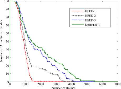
Fig.1. Number of alive sensor nodes vs. number of rounds, when m=0.48, m 0 =0.44, α=1.82, β=2.42 and θ =0.52.

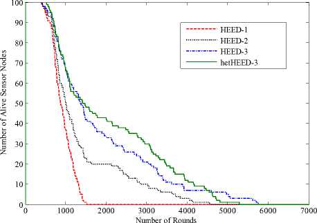
Fig.2. Number of alive sensor nodes vs. number of rounds, when m=0.45, m 0 =0.33, α=1.66, β=3.33 and θ =0.55.

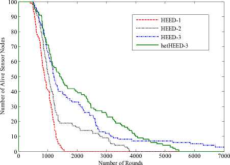
Fig.3. Number of alive sensor nodes vs. number of rounds, when m=0.42, m 0 =0.21, α=1.73, β=4.76 and θ =0.58.

Number of Rounds

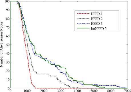
Fig.4. Number of alive sensor nodes vs. number of rounds, when m=0.40, m 0 =0.10, α=2.20, β=5.20 and θ =0.60.

However, we have shown the results for eleven cases in tables along with their parametric values for HEED-3 and hetHEED-3. The reason for showing 11 results is that we varied the model parameter θ as 0.51, 0.52,…, 0.61 obtained from (9).

As evident from Tables 4 and 5, the hetHEED-3 provides longer lifetime than that of the HEED-3 for all cases. In HEED-1/hetHEED-1 protocol, the nodes die much faster. In hetHEED-2, the nodes die slowly as compared to the hetHEED-1 due to advance nodes. In HEED-3 and hetHEED-3, the nodes die further slowly due to the advance and super nodes. However, the nodes in hetHEED-3 dies slower than the HEED-3 because it elects the cluster head in an effective manner which helps in prolonging the network lifetime.

Table 4. Network Lifetime (in Rounds) for HEED-3 protocol

Super Nodes & energy of a node	Advance Nodes & energy of a node	Normal Nodes & energy of a node	Parameters m, Шс , α, β	Network lifetime in terms of round for
				100 alive node	75 alive nodes	50 alive nodes	25 alive nodes	0 alive nodes
23 & 1.67	26 & 1.38	51 & 0.5	0.49, 0.47, 1.76, 2.34	433	876	1359	2610	4277
21 & 1.71	27 & 1.41	52 & 0.5	0.48, 0.44, 1.82, 2.42	433	870	1247	2444	4131
19& 1.81	28 & 1.41	53 & 0.5	0.47, 0.40, 1.82, 2.62	393	936	1379	2921	4773
17& 1.86	29 & 1.40	54 & 0.5	0.46, 0.37, 1.80, 2.72	380	810	1439	2967	5514
15 & 2.17	30 & 1.33	55 & 0.5	0.45, 0.33, 1.66, 3.33	433	863	1379	2444	5772
13 & 2.26	31 & 1.37	56 & 0.5	0.44, 0.29, 1.75, 3.52	459	870	1339	2583	6169
11 & 2.75	32 & 1.30	57 & 0.5	0.43, 0.26, 1.59, 4.50	420	909	1161	2682	6957
9 & 2.88	33 & 1.36	58 & 0.5	0.42, 0.21, 1.73, 4.76	502	926	1213	2431	7005
7 & 2.92	34 & 1.47	59 & 0.5	0.41, 0.17, 1.95, 4.84	442	956	1213	2695	6990
4&3.1	36 & 1.60	60 & 0.5	0.40, 0.10, 2.20, 5.20	339	843	1247	2689	6917
2 & 3.52	37 & 1.69	61& 0.5	0.39, 0.05, 2.38, 6.04	434	843	1221	2801	6998

Table 5. Network Lifetime (in Rounds) for proposed hetHEED-3 protocol

	Super Nodes & energy of a node	Advance Nodes & energy of a node	Normal Nodes & energy of a node	Parameter Θ	Network lifetime in terms of round for
					100 alive node	75 alive nodes	50 alive nodes	25 alive nodes	0 alive nodes
	23 & 1.64	26 & 1.42	51 & 0.5	0.51	453	903	1359	2974	4350
	21 & 1.68	27 & 1.45	52 & 0.5	0.52	314	810	1399	2960	5508
	19& 1.71	28 & 1.48	53 & 0.5	0.53	433	889	1485	2848	5097
	17& 1.74	29 & 1.51	54 & 0.5	0.54	433	942	1273	3288	5236
	15 & 1.77	30 & 1.54	55 & 0.5	0.55	532	883	1478	3079	5283
	13 & 1.80	31 & 1.57	56 & 0.5	0.56	539	999	1359	2815	4707
	11 & 1.84	32 & 1.61	57 & 0.5	0.57	486	936	1359	3146	6004
	9 & 1.88	33 & 1.64	58 & 0.5	0.58	502	926	1425	2998	5485
	7 & 1.92	34 & 1.68	59 & 0.5	0.59	351	850	1266	3104	5727
	4& 1.96	36 & 1.72	60 & 0.5	0.60	440	843	1353	2921	5647
	2 & 2.02	37 & 1.77	61& 0.5	0.61	434	873	1251	3308	6075
References V. Conclusion                        [1] W. Dargie and C. Poellabauer, “Fundamentals of Wireless In this paper, we have proposed a 3-level Sensor Networks: Theory and Practice,” John Wiley and heterogeneous network model characterized by a single         Sons , 2010. [2] K. Sohraby, D. Minoli, and T. Znati, “Wireless Sensor model parameter and can describe 1-level, 2-level and 3-                    ,          ,            , Networks: Technology, Protocols, and Applications,” level energy heterogeneity in a network. The energy          John Wiley and Sons , 2007, 203-209. heterogeneity helps increasing the network energy and [3] R. Szewczyk, E. Osterweil, J. Polastre, M. Hamilton, A. utilizing the network energy efficiently increases the          Main-waring, and D. Estrin, “Habitat Monitoring with network lifetime. The hetHEED-3 increases the network         Sensor Networks,” Communications of the ACM , 2004, lifetime by 299% by increasing the network by 100%         47(6):34-40. with respect to the original HEED. Thus, we have shown [4] C.Y. Chong and S. P. Kumar, “Sensor Networks: that our heterogeneous network model uses network Evolution, Opportunities and Challenges,” in proc. of the energy in effective manner for enhancing the network         IEEE , 2003, 91(8):1247-1256. lifetime.                                                     [5] W. Heinzelman, A. Chandrakasan, and H. Balakrishnan,

"Energy-Efficient Communication Protocol for Wireless Microsensor Networks," in proc. of the 33^rd Hawaii Int. Conf. on Systems Science (HICSS '00), 2000, 8:3005-3014.

• [6]    W.R. Heinzelman, A.P. Chandrakasan, and H. Balakrishnan, “An Application-Specific Protocol Architecture for Wireless Microsensor Networks,” IEEE Transactions on Wireless Communications , 2002, 1(4): 660–670.

• [7]    S. Lindsey, and C. Raghavendra, “PEGASIS: PowerEfficient Gathering in Sensor Information Systems,” in proc. of the IEEE Aerospace Conf., Montana , 2002, 3: 1125-1130.

• [8]    S. Lindsay, C. Raghavendra, and K. Sivalingam, “Data Gathering in Sensor Networks Using the Energy Delay Metric,” in proc. of the 15th Int. Parallel and Distributed Processing Symposium , 2001, 2001-2008.

• [9]    A. Manjeshwar and D. P. Agarwal, “TEEN: A Routing Protocol for Enhanced Efficiency in Wireless Sensor Networks,” in proc. of the 1st Int. Workshop on Parallel and Distributed Computing issues in Wireless Networks and Mobile Computing, San Francisco , 2001, 2009-2015.

• [10]    A. Manjeshwar and D. P. Agarwal, “APTEEN: A Hybrid Protocol for Efficient Routing and Comprehensive Information Retrieval in Wireless Sensor Networks,” in proc. of the Int. Parallel and Distributed Processing Symposium, IPDPS 2002 , 2002, 195-202.

• [11]    M. Ye, C. Li, G. Chen, and J. Wu, “EECS: an Energy Efficient Cluster Scheme in Wireless Sensor Networks,” in proc. of the IEEE Int. Workshop on Strategies for Energy Efficiency in Ad Hoc and Sensor Networks (IEEE IWSEEASN-2005), Arizona, 2005, 535-540.

• [12]    N. Eshghi and A.T. Haghighat, "Energy Conservation Strategy in Cluster-Based Wireless Sensor Networks," in proc. of the Int. Conf. on Advanced Computer Theory and Engineering , 2008, 1015-1019.

• [13]    H. Junping, J. Yuhui, and D. Liang, “A Time-based Cluster-Head Selection Algorithm for LEACH,” IEEE Symposium on Computers and Communications, ISCC 2008 , 2008, 1172-1176.

• [14]    O. Younis and S. Fahmy, “Distributed Clustering in Ad-hoc Sensor Networks: A Hybrid, Energy-Efficient Approach,” IEEE Transactions on Mobile Computing , 2004, 3(4), pp. 366-379.

• [15]    O. Younis and S. Fahmy, "An Experimental Study of Energy-Efficient Routing and Data Aggregation in Sensor Networks," in proc. of the Int. Workshop on Localized Communication and Topology Protocols for Ad hoc Networks, held in conjunction with the 2nd IEEE Int. Conf. on Mobile Ad Hoc and Sensor Systems (MASS-2005), 2005, 50-57.

• [16]    H. Huang and J. Wu, “A Probalilistic Clustering Algorithm in Wireless Sensor Networks,” in proc. of the 62nd IEEE Vehicular Technology Conf., 2005, 3:17961798,.

• [17]    A. Salim, W. Osamy, and A. M. Khedr, “IBLEACH: intra-balanced LEACH protocol for wireless sensor networks,” Wireless Networks , 2014, 20(6):1515–1525.

• [18]    J. Hong, J. Kook, S. Lee, D. Kwon, and S. Yi, “T-LEACH: The Method of Threshold-Based CH Replacement for Wireless Sensor Networks,” Information Systems Frontiers , 2009, 11(5):513–521.

• [19]    F. Bajaber and I. Awan, “Adaptive Decentralized ReClustering Protocol for Wireless Sensor Networks,” Journal of Computer and System Sciences , vol. 77, no. 2, pp. 282-292, 2011.

• [20]    M. Bsoul, A. Al-Khasawneh, A. E. Abdallah, E. E. Abdallah, and I. Obeidat, “An Energy-Efficient

  Threshold-Based Clustering Protocol for Wireless Sensor Networks,” Wireless Personal Communications , 2013, 70(1): 99–112.