Homogeneous densities clustering algorithm

Published Online October 2018 in MECS DOI: 10.5815/ijitcs.2018.10.01

Because of information technology age that we live in nowadays, most organization collect huge amount of data every day, this motivate scientists and researchers to search for methods to analyze the collected data and maximize the benefit that can be earned from these repositories of data, this lead to the emergence of data mining and knowledge discovery from data. Data clustering methods that are used to group data into subsets, each subset is called cluster. Objects within the cluster have high similarity to each other and are dissimilar to objects in other clusters. Similarity or dissimilarity is based on distance or k-nearest neighbors or shared nearest neighbors or links. The functions that can be used to calculate similarity or dissimilarity are given in Table 1. Where d refers to dimensionality of space.

There are a lot of clustering algorithms that have been proposed. These algorithms may be classified into partitioning methods, hierarchical methods, density-based methods, model-based methods, and grid-based methods [1] as shown in Fig. 1.

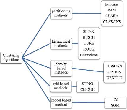
Fig.1. Classification of Clustering Algorithms

Table 1. Similarity and dissimilarity measure for interval-scaled attributes

Name of function	Mathematical formula		Comment
Minkowski Distance	dis ( X , Y ) = (£| x , - y, q ) q i = 1	(1)	q is positive real number
Euclidean Distance	dis ( X , Y ) = £ ( x , - y) i = 1	(2)	equals to minkowski diatance where q =2
Average distance	1 d             2 dis ( X , Y) = J-X( X - У . ) V d ы	(3)	is modified version of Euclidean distance
Manhattan Distance	dis ( X , Y ) = £| x , - y ,| i = 1	(4)	equals to minkowski diatance where q =1, sensitive to outliers
Maximum Distance	dis(X , Y ) = max d., |x , - y,|	(5)	equals to minkowski diatance where q ->rn
Pearson correlation	,       X ( x - x )( y.- У ) dis ( X , Y ) = -(1 -     i =1    _  ,      _  ) J X ( xi - x ) 2 X ( yi - y ) 2 V i = 1                   i = 1	(6)	used in gene expression clustering
Mahalanobis distance	dis ( X , Y ) = ( x - y ) 5 " ' ( x - y ) T	(7)	used in hyper ellipsoid clusters, S is covariance matrix
	T xT y	(8)
Cosine similarity	sum i -zX. , Y ) cos t x . X xi^ X у		used in document clustering
Chord distance	iLx.y. dis ( X , Y )   2 2 .—x_  — 1 ж	(9)	used for normalized attributes

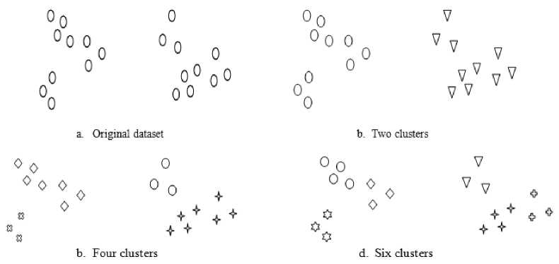
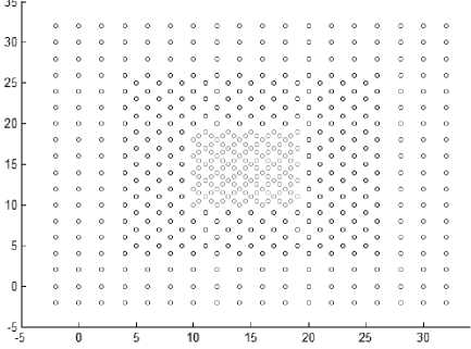
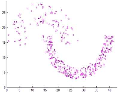
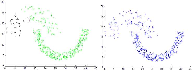
Fig.2. How many clusters in the original dataset

All portioning methods can handle data with spherical shaped clusters only and cannot handle varied shaped clusters unless they are well separated. Also, they cannot handle overlapped clusters. In addition to they require number of clusters in advance, and this is another problem. See the following Fig. 2, how many clusters in this dataset? There is more than one answer shown in Fig.

• 2.    The answer depends on the required result, the type of

the clustering algorithm used, in addition to the definition of required clusters, and the metric measure used by the algorithm. This motivates researchers to search for other clustering categories like hierarchical and density-based methods.

Hierarchical methods generate a dendrogram like a tree structure representing the clustering process. The dendrogram can be generated from bottom up as in agglomerative methods or can be generated from top down as in divisive methods [1]. Agglomerative methods are more famous than divisive methods. In single link algorithm [5] (Agglomerative method), each object in the input dataset is considered as a singleton cluster, in each step the algorithm selects the two most similar clusters to merge them until all objects are in the same cluster or level of dissimilarity is reached or required number of clusters is reached. Disadvantages of the hierarchical methods is that any step cannot be backtracked or undo, also these methods require o( n ²), there is no objective function to be minimized as in partitioning methods. Advantage of hierarchical methods is their ability to discover varied shaped clusters. Examples for algorithms in this category are average link [6] and complete link [7], CURE (Clustering Using Representatives) [8], BIRCH (Balanced Iterative Reducing and Clustering using Hierarchies) [9], CHAMELEON [10], and ROCK. (RObust Clustering using linKs)[11]. ROCK algorithm is dedicated to deal with Boolean and categorical attributes.

Density-based methods have introduced a new definition for clusters; where clusters are recorded as dense regions separated from each other by sparse regions. The density of object here may be computed as the number of objects in its neighborhood radius as in DBSCAN [12] algorithm which is a pioneer algorithm in this category, OPTICS (Ordering Points To Identify the Clustering Structure) [13] is another algorithm which is an extension of DBSCAN but it doesn’t produce clusters explicitly. Another algorithm is DENQLUE (DENsity based CLUstEring) [14].

Grid based methods, instead of applying clustering on data objects directly; they house data objects in grid cells by partitioning each dimension into finite number of cells of equal length. Then compute some statistical information about objects in each cell; such as number of objects, average mean of objects, standard deviation, and some other information as described in STING algorithm [15].

Here we propose an effective idea to improve the results of DBSCAN algorithm. This idea allows the algorithm to control the density within each cluster, by allowing small variance in density within a cluster. The proposed algorithm uses two input parameters; the first one allows the algorithm to adapt the Eps in each cluster, and the other is minpts as in DBSCAN. This paper is organized as follow. Section 2 reviews some of the previous work related to the proposed method. The proposed method is presented in section 3. Section 4 shows some experimental results of the proposed method and we conclude with section 5.

• II.    Related Work

In this section we review some algorithms related to the proposed one. First, we review DBSCAN algorithm, which is the pioneer algorithm.

• A.    DBSCAN algorithm

DBSCAN is the most famous clustering algorithm that can find varied shaped of varied size clusters. It has a trouble in handling varied density clusters; this problem results from its dependency on the global user input parameter neighborhood radius which called Eps , it requires other input parameter called minpts ; these two parameters judge the process of finding clusters. We see the problem arise because the algorithm concentrates only on minimum density allowed within a cluster and ignores the maximum density allowed within it. It allows any core point to expand the cluster without any top limitation on density. So, it allows large variance in density within a cluster. If we need to discover clusters of varied density we must search for a method to control the maximum density allowed within the cluster, this is what this paper propose. DBSCAN depends on some basic definitions as follow: -

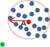
• 1.    Eps -neighborhood of a point x denoted by N_Eps( x ) ={y е Dataset | dis( x , y ) ≤ Eps }. Look at Fig. 3.

• 2.    Point x is directly density reachable from point y with respect to Eps and minpts if:-a. x ^е NEps ( y ).

• b. | N Eps ( y )| ≥ minpts.

• 3.    Point x is density reachable from y with respect to Eps and minpts if there exist a chain of points z ₁, z ₂,…, z _n. Where y = z ₁ and x = z _n, such that each point in the chain is direct density reachable from the previous one as shown in Fig. 4.a; this relation is not always reversible, as you see in Fig. 4.a, x is density reachable from y but y is not density reachable from x since x is border point. However, if x and y are core points then they are density reachable from each other.

  N

  
  
  
  
  

  N•

  

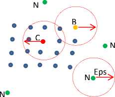
  Fig.3. Type of points A and C are core points, B is border point, points labeled N are noise points, red arrow represent Eps, minpts = 4.

  
  

• 4.    Point x is density connected to y with respect to Eps and minpts if there exist point z such that x and y are density reachable from z with respect to Eps and minpts . As shown in Fig. 4.b , two points x

• 5.    Cluster is non-empty subset of the input dataset with maximality and connectivity

All points that reside in the Eps neighborhood radius of the red point (core point A or C) are directly density reachable as shown in Fig.3.

and y are density connected if there is a chain of core points connecting them.

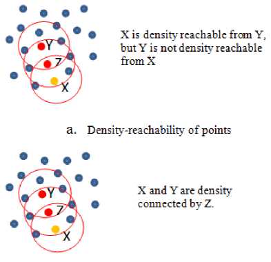
b. Density connectivity of points

Fig.4. Density reachability and connectivity.

• a.    if x e C and y is density reachable from x with respect to Eps and minpts then y e C.

• b.    if x ■= C and y e C then x is density connected to y with respect to Eps and minpts .

• 6.    Noise is a set of points that are not belonging to any cluster. See Fig. 3, noise point does not belong to any neighborhood radius of core point and have number of points in its Eps radius less than minpts .

Based on the previous definitions DBSCAN cannot handle datasets shown in Fig. 5 due to the presence of varied density clusters that are very close to each other. Any cluster consists of core points and border points. Noise points are discarded and will not belong to any cluster. The DBSCAN algorithm is described as follow: -

DBSCAN(data, Eps , minpts )

Clus_id=0

FOR i=1 to size of data

IF data[i] is unclassified THEN

IF (|NEps(data[i])|≥ minpts ) THEN

Clus_id=clus_id +1

Expand_cluster(data, data[i], Eps , minpts , clus_id)

ENDIF

ENDIF

NEXT i

All unclassified points in data are noise

End DBSCAN

Expand_cluster(data, data[i], Eps , minpts , clus_id) Seed=data[i].regionquery(data[i], Eps )

Data[i] and all unclassified points in seed are assigned to clus_id

Seed. delete(data[i])

While seed<> empty do

Point=Seed.getfirst

Neighbor= point.regionquery(point, Eps )

Append all unclassified points in neighbor to seed and assign them to clus_id

ENDIF

End while

End Expand_cluster

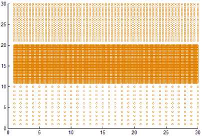
Dataset1

Dataset2

Fig.5. Datasets with very close varied density clusters.

There are many researchers tried to enhance DBSCAN algorithm to handle varied density clusters, we review some of their works in next subsection.

• B.    Varied densities clusters

Here, we review some of recent researches discussed the problem of multi-density clusters. In DVBSCAN [16], it is based on DBSCAN and add two more threshold to control clustering process; they are cluster density variance and cluster similarity index. The resulting clusters of DBSCAN algorithm is very sensitive to small change in Eps , and the authors introduce two more parameters that impact on the result. Tuning of four parameters is very hard task.

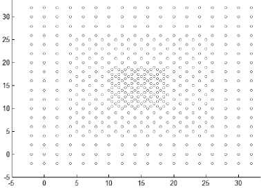
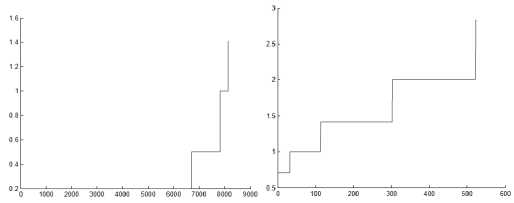
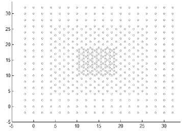
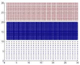
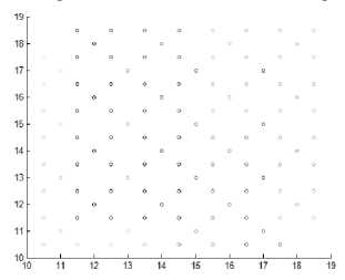
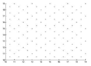
In DMDBSCAN [17], the authors select several values for the neighborhood radius Eps from the k-dist plot. They checked the k-dist plot by their eye depending on seeing sharp change in k-dist curve, and this is not always true because of the presence of noise and outlier points. Examine Fig. 6, this is true for the first dataset shown in Fig. 5 where you can see three levels of density within the dataset1. For the second dataset shown in Fig. 5, you see four levels of density, but the dataset2 shown in Fig. 5 contains only three clusters of different densities, and this lead to split the densest cluster. For the third dataset shown in Fig. 8, you see only one level of density in k-dist plot shown in Fig. 6 but examine the dataset itself you see at least three levels of density. For the fourth dataset shown in Fig. 8, you see many small changes on the curve in Fig. 6, this may lead to find large number of clusters, but the dataset contains two clusters of varied densities.

Dataset1

Dataset2

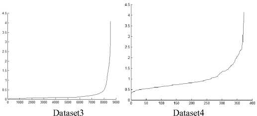
Fig.6. 3-dist plot for the first four datasets in experiment

In [18] the authors propose to use spline cubic interpolation to find suitable values for Eps from the curve of k-dist plot. By using the interpolation, they find mathematically the inflection points of the curve where the curve changes its concavity and these points correspond to Eps values that will be used in DBSCAN. But this may lead to split some clusters. For example, see 3-dist plot of dataset 2 in Fig. 6, you find seven inflection points that split the densest cluster, in 3-dist plot of dataset 4 also you find many of inflection points, this lead to get large number of clusters. And for the third dataset, there is only one inflection point.

In K-DBSCAN [19], the authors use k-means algorithm to divide points into different density level to identify the corresponding densities in dataset, they calculate the density of point as the average sum of distance to k-nearest neighbors, and sort these distances, and from the density curve checking sharp change in density to determine the value of k in k-means. Then apply a modified version of DBSCAN algorithm in each level of density. The result depends on density levels result from the k-means. The average distance to k-nearest neighbors is similar to k-dist plot, and the algorithm suffer from seeing incorrect multiple level of densities as in [17,18]. In [20] the author has introduced a framework to handle varied density clusters.

• III.    The Proposed Method

The main problem of DBSCAN algorithm is the large variance in density allowed within the cluster, this problem arise due to its global user input variable that is called Eps, it is very difficult to depend on single value for this parameter, most datasets contain clusters with varied densities, if the value of Eps is small the DBSCAN algorithm discovers only most dense clusters and low density clusters will be discarded as noise points, on the other hand if the value of Eps is large enough to discover low dense clusters this may lead to merge some of dense clusters of different densities unless they are well separated by sparse regions. To solve this problem, we set maximum value for density allowed within the same cluster. i.e the neighborhood of any core point must contain number of points greater than or equal to minpts and smaller than or equal to maxpts.

When using the k-nearest neighbors you see that the neighborhood radius is small in dense regions and is large in sparse regions. This means, there exist reverse proportional between neighborhood radius and density of region, as the density increase the radius decrease and the vice versa. In the proposed method as the difference between the maxpts and minpts increase, the variance of density within the cluster increase. When the difference decreases the variance of density within the cluster decreases, this is a proportional relation between the difference between maxpts and minpts and the density variance within the clusters.

The DBSCAN depends on k -dist plot where k = 4, that represent the low level of density for any core point. The proposed algorithm will depend on k -dist plot, where k = maxpts , that represent the maximum level of density for any core point. Depending on this idea the algorithm uses the distance to the maxpts neighbors as neighborhood radius for the region where this core resides, and the algorithm expands the current cluster by visiting all density reachable core points with respect to minpts , maxpts and Epscr (EPS of current region). As the difference between maxpts and minpts decrease the algorithm return as a result large number of homogenous clusters, whereas the difference between maxpts and minpts increase the algorithm return small number of lower homogenous clusters.

The proposed algorithm will depend on the following definitions: -

• 1-    Initiator of cluster is the core point that has the minimum neighborhood radius among all unclassified point and has maxpts of points within its neighborhood radius.

• 2-    The density of any core point p satisfies this relation: minpts ≤ |N_Epscr (p)|≤ maxpts .

• 3-    Point p is direct density reachable from q if p Е N_Epscr ( q ), q is core wrt. Minpts , maxpts , and Epscr .

• 4-    Other definition is the same as that of DBSCAN algorithm in addition to handle the duplicated points as a single point.

Now we present the details of the proposed algorithm that will be called HDCA (Homogenous Density Clustering Algorithm). This algorithm requires only two input parameters; they are minpts and maxpts that control minimum and maximum density allowed within the cluster. Also, the algorithm uses the maxpts to find the appropriate value for the neighborhood radius of the current region, it refers to this value as Epscr. Here, cluster is defined as a region that has points of homogenous density satisfying maximality and connectivity conditions.

To find clusters in the input dataset D of N points, the algorithm arranges the points in ascending order based on their distances to maxpts . So, the first data point in the ordered dataset is the initiator of the first cluster, and the distance to the maxpts is the value of Epscr (neighborhood radius of current region), the algorithm starts to expand the current cluster wrt. minpts , maxpts and Epscr until no point can be added to it, then it moves to the next unclassified point, this leads to set the distance of its maxpts neighbor to Epscr and expand cluster with ignoring previously classified points. Very small clusters may be ignored in the result. The following lines describe the proposed algorithm.

HDCA(dataset, minpts , maxpts )

Find distance to maxpts

Next i

Clusid = 0

Sort points based on the calculated distance to maxpts in ascending order

If p[i].Clusid = unclassified then

Clusid+ = 1

Expand_cluster(dataset, i , minpts , maxpts , Clusid)

Endif

Next i

End HDCA

Expand_cluster(dataset, i , minpts , maxpts , Clusid) Epscr = p[i].dis[maxpts]

Seed = regionquary(p[i], Epscr)

All unclassified points in seed and p[i] are assigned to Clusid

Curpt = seed.getfirst()

Newseed = regionquary(Curpt, Epscr)

All unclassified points in Newseed are appended to seed

All unclassified points in Newseed are assigned to Clusid

Endif

Endwhile

Else

P[i] is classified as noise temporary

Endif

End Expand_cluster

• IV.    Experimental Results

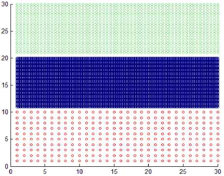
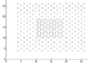
  This section shows the result of applying the proposed method to some synthetic dataset containing data in twodimensional space to visualize the result easily. We have used different datasets containing clusters of varied densities, shapes, and sizes. The proposed method succeeded in discovering clusters even though the high closeness of each other. The first two datasets used in the experiment are shown in Fig. 5, the first dataset has 8137 points in three clusters of varied density which are very close to each other and cannot be discovered by DBSCAN algorithm based on single global value for neighborhood radius. The second data set has 526 points, in three varied density clusters. The problem here is more difficult because each cluster is surrounded by another cluster of different density; the central cluster is the densest one which immediately surrounded by dense cluster without separation which are surrounded by sparse cluster, and the algorithm detects the clusters correctly as shown in Fig. 7

Dataset1

Dataset2

Fig.7. Result from applying the HDCA method on datasets shown in Fig. 5.

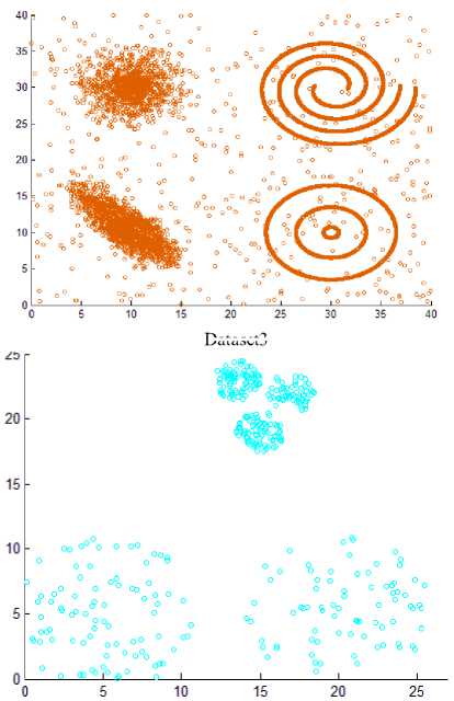
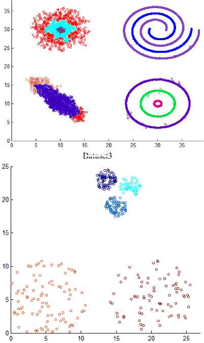
Dataset3

Dataset5

Dataset4

Dataset6

Fig.8. Other datasets that are used in experiments

Dataset3

Dataset5

Dataset4

Dataset6

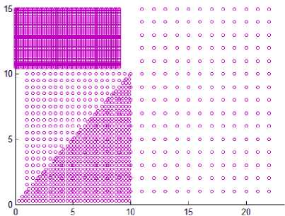
Fig.9. Result from applying the HDCA method on datasets shown in Fig. 8.

6. Eps=1.5 to 1.9

7. Eps=2

3. Eps=1.1

4. Eps=0.8

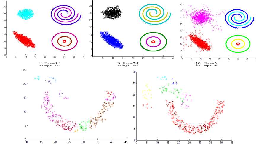
8. Eps=0.4

9. Eps=0.5

10. Eps=2

11. Eps=1

12. Eps=2

5. Eps=1 to 1.3

13. Eps=3.5

14. Eps=4

Fig.10. The resulting clusters from applying DBSCAN on the datasets using different values for Eps.

As the difference between maxpts and minpts increase the algorithm allow cluster to increase the density variance within it, as a result the number of clusters will decrease. The other datasets that are used in experiments are shown in Fig. 8. Dataset 3 has 8573 points distributed over varied shaped, sized and density clusters with the presence of noise points, there are two intertwined spiral clusters, and three ring clusters each one surrounds the others, these five clusters are of the same density, there are other two clusters have large variance in density, the algorithm extracts homogeneous clusters from them. Dataset 4 has 373 points distributed over two clusters of different density. Dataset 5 has 383 points in five spherical shaped clusters with two level of density. Dataset 6 has 3147 points in four clusters of different densities with no separation among them.

Fig. 9 shows the resulting clusters from applying the HDCA algorithm on the datasets in Fig. 8. These results show the efficiency of the algorithm in extracting homogeneous clusters from the data.

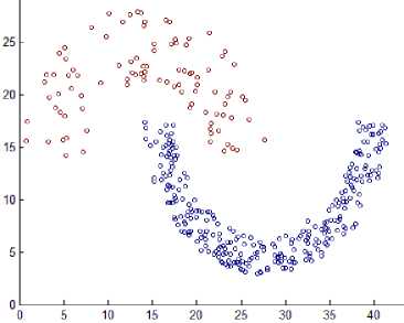
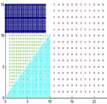
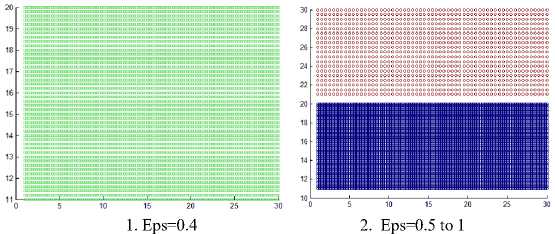
Fig. 10 shows the resulting clusters from applying the DBSCAN algorithm on the first four datasets that are shown in Fig. 5, 8 comparing these results with that of the proposed HDCA algorithm in Fig. 9, you note that the DBSCAN algorithm failed to find the homogenous clusters from the data. It fails to discover the actual clusters in dataset 1, 2, 3, 4 because of the presence of varied density clusters, and in dataset 3 when Eps = 2 as in Fig. 10.10 the two left clusters surrounded by sparse points, but these sparse points assigned to them, and this make each of them allow large variance in density. When Eps = 0.5, become smaller it discards the sparse points, and all clusters are of the same density. When Eps = 0.4, the smallest value used, it discards some border points from the two left clusters as shown in Fig 10.8-10.10.

For the first dataset, when Eps = 0.4 it discovers only the densest cluster and other points considered as outliers. When Eps ranges from 0.5 to 1, it discovers two clusters because there is a sparse region separating them and removes the third cluster as outliers, when Eps = 1.1, it merges the densest cluster with the sparser one because there is no sparse region separate them, all this information is shown in Fig.10.1-10.3.

For the second dataset, see Fig. 10.4-10.7, this is the most challenging dataset since clusters are very close to each other and contained within each other. When Eps =

0.8, it splits the densest cluster to 32 clusters, when Eps ranges from 1 to 1.3 it discovers the inner densest cluster, when Eps ranges from 1.5 to 1.9 it merges the two inner clusters, when Eps =2 it doesn’t perform any clustering because it assigns all points to the same cluster, it fails to discover the correct clusters for any value of Eps , this is the main problem of DBSCAN algorithm that is solved by the proposed HDCA algorithm.

For the fourth dataset, it is also challenging dataset. It contains two clusters that cannot be discovered by DBSCAN algorithm for any value for Eps as shown in Fig. 10.11-10.14, when Eps =1 it splits the two clusters and produces 12 clusters, when Eps = 2 it finds the denser cluster but splits the sparser one to six clusters to get seven clusters as a result. When Eps = 3.5, it discovers two wrong clusters, it splits the sparser one and merges one part of it with the denser cluster. When Eps = 4, it assigns all points to the same clusters.

Note that all values used for Eps in DBSCAN algorithm are taken from the 3-dist plot shown in Fig. 6.

• V.    Conclusion

Reviewing the DBSCAN algorithm, it is very interesting algorithm, it can handle clusters with varied shaped and sized but fails to handle clusters of varied density because of its global variable Eps , the proposed method tries to handle this problem by allowing homogeneous density connected cores to be grouped in one cluster. To achieve this; the proposed method determines maximum level of density allowed within each cluster, and this allows DBSCAN to use varied values for Eps according to the density of region. The experimental result revealed the ability of the proposed method to handle clusters with varied density. When comparing the results, we get from both algorithms on the same datasets, we find that the proposed algorithm easily discovered the actual clusters in the datasets.