How do Machine Learning Algorithms Effectively Classify Toxic Comments? An Empirical Analysis

Published Online on August 8, 2023 by MECS Press

Nowadays, discussion over online platforms is a familiar and easy way of communication. The platforms provide the facility to discuss various trending topics, share information and views, etc., over a topic. However, maintaining a healthy environment and good conduct over these platforms is difficult. Lots of malicious, harassing, insulting, jeering, toxic, and cyberbullying activities have become very common on such platforms [1], which negatively affects online users. As a result, some people stop giving their opinions or seek different opinions, resulting in harmful and unjust discussions. Consequently, online service providers need help solving this problem. They are often forced to limit user comments or get dissolved by shutting down user comments completely. Social media service providers have worked on different solutions to overcome the challenges, such as comment classification techniques, user blocking mechanisms, and comment filtering systems.

The toxic comment classification system involves classifying the comments based on their toxicity levels into predefined classes. By categorizing the comments into various labels, the service providers can take necessary actions to control the occurrence and growth of the negative influences created by such activities on online platforms. This type of comment classification system will ensure the purpose of social conversation is more effective and positive. To this end, an automatic comment filtering system is essential to save time and manual efforts in controlling toxic comments on online platforms. As an automatic toxic comment detecting effort, the cyber hate was identified individually and intersectionally using linear Support Vector Machine (SVM) and random forest decision tree algorithms [2]. The toxic comment classification was introduced to investigate the benefits of using a Convolutional Neural Network (CNN) [3]. The effect of automatic feature engineering for hate speech detection using LR and linear SVM was analyzed by [4]. The challenges for toxic comment classification were demonstrated using LR, bidirectional Recurrent Neural Network (RNN) and CNN [5]. Prediction gains of traditional shallow learning for toxic comment classification are analyzed empirically in [6].

The adversarial text input was generated by [1] to assess its effectiveness against Google's Perspective toxic comment classifier. The LR, CNN, Long Short-Term Memory (LSTM), and Conv + LSTM-based toxic comment classifiers were suggested by [7]. The problem of dealing with imbalanced datasets in toxic comments classification was solved using data augmentation and deep learning techniques [8]. The gradient boosting-based toxic classification was performed by [9]. The unstructured text is classified into toxic and non-toxic using naïve bayes, LSTM and RNN [10]. The research [11], defined toxicity-initiating actions in online discussions as non-toxic comments that lead to toxic replies applying several algorithms. Empirical analysis of shallow and deep learning models for toxic comment detection was conducted [12]. Utilizing LR, neural network and LSTM models, the source of bias in toxicity classifiers is resolved [13]. On the other hand, the performance of LR, SVM and bidirectional LSTM was investigated by [14]. The hate speech was detected using the Bidirectional Encoder Representations from Transformers (BERT) [15]. To compare the performance of different techniques, six ML algorithms were combined with N-grams, linguistic and lexicon features for French toxic comment categorization [16]. CNN and bidirectional Gated Recurrent Unit (GRU) was presented by [17] for classifying different types of toxicity. Furthermore, the negativity and toxicity in online comments were also analyzed in [18] to filter those who harass others leveraging LR, Naïve Bayes (NB), and Decision Tree (DT). In the literature, several ML classifiers were investigated e.g. LR [11-14, 16, 20], NB [3, 18], SVM [2-4, 14, 16], k-nearest neighbors [3, 16], DT [11, 16, 18], random forest [2, 11, 16], and AdaBoost [11], on top of those algorithms, we have experimented ridge, passive-aggressive, stochastic gradient descent, bagging and gradient boosting to view the toxic comment classification broadly.

Unfortunately, the classifiers do not perform well with all feature extraction systems for toxic comment analysis. The perfect selection of ML algorithm and feature extraction strategy is essential to get excellent classification performance. In this context, exploring the best combination of an ML algorithm and feature extraction technique for toxic comment analysis is significant research. Therefore, this research will conduct experimentation with 15 supervised ML algorithms with four feature encoding schemes. ML algorithms will detect six toxicity types i.e., toxic, severe toxic, obscenity, threats, insult and identity hate in the textual data. The classifier will predict whether an input text is either toxic or non-toxic. The main objective of this paper is to find the best pair of an ML algorithm and feature extraction strategy to classify toxic comments. For that, the toxic comment classification model needs to be built, which must be capable of reading the textual comments. Also, it needs to split the comments into different classifications. Finally, the model must identify the different toxicity types in the textual comments. The paper addressed 4 Research Questions (RQ) to explore the best combination of ML algorithms and featuring schemes for toxic comment detection.

RQ1: What is the distribution of toxicity types in online behaviors? The dataset can be analyzed to view the class (label) distribution. Counting and comparing the number of comments under each class can demonstrate the different toxicity distributions, which need counting both the all-comments and only toxic comments. The calculated records show that 16225 out of 159571 comments (10.17%) are identified as some sort of toxic. Where only 39% of the toxic comments have only one label, and the majority have some overlap.

RQ2: How do feature extraction strategies differ based on ML algorithms in toxic comment classification? Four feature extraction strategies with word level n-grams, character level n-grams and character word bound options are investigated for several ML algorithms. Each classifier will be needed to apply all featuring schemes. In the experiment, the classifier performance is varied based on the different feature sets. We have found that, out of the four investigated featuring options, TF-IDF has the top average score of 0.809 (roc-auc).

RQ3: Which ML algorithm group is preferred to work on toxic comment classification? The selected ML algorithms are clustered into several groups based on their similarity of application, named Regression, Bayesian, Instance-based, Decision Tree and Ensemble. We observed that Regression group algorithms performed better than any other individual group.

RQ4: Which ML algorithm outperforms for classifying toxic comments in online behaviors ? The outcome of each ML model will be evaluated based on the evaluation metrics accuracy and roc-auc. We have concluded that the best performers of toxic comment classification are LR and AdaBoost, with an average accuracy of 0.895 and 0.893, respectively.

2.    Related Works

Toxic comment analysis is a significant problem in online social media platforms. Because of its importance in practice, several types of research have been conducted using various ML algorithms to detect toxic comments. The relevant research work concerning toxic comment analysis is summarised in this section.

Ain et al. proposed a method to generate adversarial text input and assess its effectiveness against Google's Perspective classifier [1]. A targeted attack scheme was designed to make Perspective misclassify toxic comments as clean. A surrogate model was trained to emulate Perspective's decision boundaries and applied existing attacks on this system. Then, a list of text candidates is generated by discretizing the adversarial features. The system includes a text candidate-generating process from perturbed features and selects candidates to retain syntactic similarity. The classifier can be deceived by replacing words in toxic sentences while preserving the original meaning.

Burnap et al. built generalizable machine-learning models to identify different types of cyber hate individually and intersectionally [2]. The proposed model addresses the intersectionality challenge by providing evidence to support the hypothesis that classification can be improved by developing a blended model. It uses text parsing to extract typed dependencies, representing syntactic and grammatical relationships between words. In addition, a data-driven blended cyber-hate model was developed to improve classification where more than one protected characteristic may be attacked. Linear SVM and random forest decision tree algorithms performed the experimentation.

Georgakopoulos et al. proposed a CNN-based approach for toxic comment classification [3]. The study investigated the benefits of using CNN in text mining using word embeddings to encode texts over the conventional classification approaches using BoW representation. Word embeddings and CNN are compared against the four BoW approaches and linear discriminant analysis, and it concludes that the CNN outperformed the BoW approaches.

Robinson et al. analyzed the effect of automatic feature engineering on ML-based methods for hate speech detection [4]. Three types of features; (i) surface features (ii) linguistic features and (iii) sentiment features are used for experimentation. The scheme used logistic regression with L1-regularization to calculate feature scores and select features based on a threshold value. Using the selected features, the linear SVM model was built to classify hate speech. The findings show that automatic feature selection can drastically reduce the carefully engineered features by over 90%. However, automatically selected features performed better classification than carefully crafted task-specific features.

Aken et al. investigated LR, bidirectional RNN and CNN to resolve the common challenges for toxic comment classification [5]. Where pre-trained Glove and sub-word embeddings were applied for feature engineering, it shows that the models make different errors and can be combined into ensembles with improved F1-measure. According to the paper, the ensembling system performs better for high-variance data and classes. Wikipedia talk pages' dataset and Twitter dataset have been utilized for this study.

Rybinski et al. empirically analyzed the predictive gains concerning traditional shallow learning models for toxic comment classification [6]. In addition, the impact of using text embedding methods and data augmentation techniques is investigated. The performance of oversampling and the gains per class yielded by data augmentation and embedding were inspected. It claims that LR can obtain competitive results compared to costly deep learning models.

Saif et al. proposed a toxic comment classification framework using LR and neural network models [7]. The neural network models include CNN, LSTM, and CNN + LSTM. The paper concluded that all experimented models solved the toxic comment classification well. However, the combined model CNN + LSTM performed best.

Ibrahim et al. implemented a multi-label approach to categorize toxic imbalance comments using data augmentation and deep learning techniques [8]. The paper solves the class imbalance problem in a dataset exploiting data augmentation schemes to generate new comments for the minority classes. Firstly, the paper uses a binary classifier to determine whether a comment is toxic or non-toxic. Secondly, another predictor identifies the toxicity label present in the tested comments. The solution considered CNN, bidirectional LSTM and GRU as classifiers. The paper claimed that the evaluated strategy outperforms all the other considered models.

Osama proposed a model to identify the toxic commenting bot on Arabic social media sites [9]. The toxic comments are identified and classified into different classes in this process. Next, the negative comments creator bot is identified. Gradient Boosting (GB) was used for performing the classification task. The dataset for this experiment is created by collecting posts and tweets from social media websites such as Facebook, Twitter, Instagram, WhatsApp, etc. The accuracy of eXtreme GB was more than 98%.

Zaheri et al. proposed a novel approach to classify unstructured text into toxic and non-toxic using supervised ML models, including NB, LSTM and RNN [10]. According to the results, the LSTM reports a 20% higher true positive rate than the naïve Bayes model. 159,000 crowd-sourcing text comments were used as a dataset in this study. The work incorporates Amazon Web Service to improve their working pipeline and demonstrated that a practical data science solution is more than an algorithm and that the architecture's scalability must be considerate of the task at hand.

Almerekhi et al. defined toxicity as initiating actions in online discussions that lead to toxic replies [11]. The text and context features are exploited in order to predict whether a given comment is a toxicity trigger. Where, the context refers to the discussion that happened before that comment. The framework experiments decision tree, random forest, adaboost and LR. In addition, fine-tuned BERT and LSTM pre-trained word embeddings from GloVe have been experimented. However, an RF model is used to classify, ranking and selection of toxic comment features.

Vaidya et. al. empirically analyzed several toxic comment detection algorithms with the focus of reducing model bias [12]. The biases of models on terms gay, lesbian, bisexual, transgender, black, Muslim and Jewish has been improved. Multi-task learning model with an attention layer has been applied to predict the toxicity of a comment. They compared shallow and deep learning models to test for unintended model bias.

Reichert et al. proposed a framework to resolve sources of bias in toxicity classifiers [13]. The framework uses several models including LR, neural network and LSTM, to classify the toxic comment. The over-sampling and undersampling strategies have been applied to balance the dataset. Textual features have been extracted using TF-IDF and Glove techniques. It compares the performances for classification and mitigation of unintended bias.

Rastogi et al. investigated the classification performance of machine learning algorithms for a small dataset utilizing a combination of data augmentation techniques [14]. The LR, SVM and bidirectional LSTM have experimented with easy data augmentation and back translation techniques to investigate their research goal. The research found that data augmentation techniques are good for boosting the performance of models significantly.

Alonso et al. proposed a hate speech detection technique applying a 5-fold ensemble training method of the RoBERTA model [15]. In this study, the RoBERTA, a variant of BERT from the Simple Transformers library, is used to tweet classification and regression. The experimental results on the HASOC tweet dataset showed that the proposed ensemble is capable of attaining state-of-the-art performance. The implemented ensemble achieved a weighted F1-score of 0.8426 and attained 0.8504 with the improved model version.

Boudjani et al. proposed an ML approach for French toxic comment classification using N-grams, linguistic and lexicon features [16]. They compared English and French results using the same method and investigated to what extent insulting in French, and English can have the same characteristics for toxic comment identification. Linear SVM, DT, random forest, LR, k-nearest neighbors and neural network algorithms were used for this investigation. The dataset has been collected from Youtube comments posted on several videos. The paper concluded that adding lexicon and linguistic features to N-grams features does not increase precision; however, it increases recall and F1-score.

Beniwal et al. demonstrated a hybrid deep-learning model to detect and classify toxic comments according to the type of toxicity [17]. The multi-label classification was built using CNN and a bidirectional GRU. In addition, the probability for each subtype has been estimated to make the model strong enough to outperform Perspective API's current models. It achieved 98.39% and 79.91% accuracy and F1-score.

Husnain et al. analyzed the level of negativity and toxicity in online comments in order to filter those who harass others [18]. First, this scheme trained the separate classifiers against each facet of the toxicity in comments, then dealt with the problem as a multi-label classification problem. Where LR, naïve Bayes, and decision tree are utilized. Here, the LR model turns out to be a better performer for both the binary and the multi-classification.

Carta et al. proposed an ML approach to solving toxic comment classification problems utilizing the Apache Spark framework [20]. Firstly, the work compares the classification performance with and without state-of-the-art word embeddings data representation. Secondly, the model's performance has been evaluated by applying word embeddings from users' comments about the Udemy e-learning platform. They report Udemy embeddings outperformed other word embeddings. This clearly indicates that word embeddings made by a closer domain taken into account improve the classification performance. The multi-task, multi-label toxic comment classification performance has been evaluated using logistic regression model.

Risch et al. describe the toxicity concept and characterize its subclass into five different toxicity classes, including (i) Obscene Language/Profanity, (ii) Insults, (iii) Threats, (iv) Hate Speech/Identity Hate and (v) Otherwise Toxic [21]. It explains that sentiment analysis support in moderation and also help to understand the dynamics of online discussion. The study presents various deep learning approaches, including datasets and architectures, tailored to sentiment analysis in online discussions. In addition, the research augmented training data by using transfer learning. The real-world applications of semi-automated comment moderation and troll detection systems have also been analyzed.

In the literature, several classifiers have experimented with toxic comment analysis. However, the classifiers only work well with some feature extraction techniques for toxic comment classification. In this context, exploring the performance of ML algorithms with different feature encoding strategies is an important research direction.

3.    Methodology

This study aims to investigate classification performance of ML algorithms combined with several feature extraction techniques for toxicity analysis in textual comments. To do so, 15 ML classifiers specifically trained for toxic comments with four feature encoding schemes. The whole working process is divided into the following three steps.

• •    Dataset Collection and Pre-processing

• •    Feature Extraction

• •    Classification Algorithms

• 3.1.    Dataset Collection and Pre-processing

• 3.2.    Feature Extraction

The details regarding the above steps are described in the following sub-sections.

The Kaggle toxic comment dataset is collected and analysed to satisfy the RQ1. This RQ tries to find out the class distribution in the dataset. For this purpose, the number of comments belonging to each toxicity type is calculated; number of both toxic and non-toxic comments for each class. Number of only-toxic comments under each class is presented also.

After the exploratory analysis, comments are cleaned and prepared to NLP pipelines. This includes noise removal, tokenization, normalization. Noise removal is a technique that is involved with removing unwanted information such as punctuation and accents, special characters, numeric digits, etc. The breaking of the text into a smaller component is called tokenization and the individual components are called token. The next step is normalization, which is the process of transforming a text into a standard form that include case-folding, stop-word removal, stemming and lemmatization. Stop words refer to the most common words such as "a", "an", "the", which do not influence the semantics of a toxic comment. The stemming bluntly removes word affixes (prefixes and suffixes). The lemmatization approach is utilized to get a base form of word and grouping the inflected words together. Lemmatization is similar to stemming but it tries to transform the word appropriately. In the end, part-of-speech tagging is used to improve the performance of the lemmatization step.

After the text pre-processing is completed, the textual features are extracted and classified based on the requirements of the RQ2. This step involves extracting several types of feature representations and then applying those features on considered ML algorithms. The ML algorithms learn from a pre-defined feature set of the training data to produce output for the test data. However, the algorithms cannot work on the raw text directly. Therefore, feature extraction techniques are used to convert textual data into a matrix (or vector) of features. As requirements of RQ2, several features are extracted from the trained dataset. The techniques include BoW , TF-IDF , Hashing and CHI2 , which are described below.

Bag of Words (BoW): This scheme maintains a bag containing all the different words present in the dataset. This bag is also known as a vocabulary dataset. Counts of each word present in the bag become the features of all the comments present in the dataset. An example of BoW with two sentences is given below (Table 1).

• S1:    He is a social boy. She is also social

• S2:    Nazmul is a social person.

Table 1. Example of BoW

	he	she	social	boy	Nazmul	person
S1	1	1	2	1	0	0
S2	0	0	1	0	1	1

Term Frequency-Inverse Document Frequency (TF-IDF): The BoW for the dataset is transformed into a matrix whose every element is a product of TF and IDF. The TF is defined as the ratio of the number of times a term (word) appears in a comment to the total number of terms in the comment. The TF is measured with “1”.

TF_t =

t _ appear _ in _ a _ document total terms in the document

The IDF is calculated as the number of the documents in the dataset divided by the number of documents where the specific term appears. This is a statistical approach used for measuring the rareness or importance of a term in the document. While TF considered all words equally important, the IDF weights down the frequent terms and scales up the rare ones as “2”.

IDF_t = log e (

total _ number _ of _ documents t _ containing _ documents

If a word is common and appears in many documents, TF-IDF will approach 0. Otherwise, it will approach 1. In this process, words are given weight in TF-IDF to measure relevance, not frequency.

Hashing: This feature vectorizing scheme converts textual features into a sparse binary vector or matrix. This is extremely efficient by having a standalone hash function and does not require a pre-built dictionary of possible categories to function. If categorical vector size is x , the encoded vector size is y and hash1 and hash2 are hash functions, the encoding will be: for each categorical variable v , (i) find the index into encoding vector i as hash1 ( v ) % y and (ii) add 1 or -1 to the encoding vector element at index i from step-(i) based on hash2 ( v ) % 2. The y represents encoding vector size which is picked according to desired output dimensionality.

Chi Squared (CHI2): Two events independency is measured through CHI2 test in statistics, which is used in feature selection to test whether the occurrence of a specific term and class are independent. The CHI2 statistics can be calculated between every comment (feature variable) and the target variable (class label) to observe the existence of a relationship between the variables and the target. If the class label is independent of the comment, we can discard that comment, otherwise the comment is very important and will be considered.

• 3.3.    Classification Algorithms

On completion of feature extraction, the comments are classified to fulfil the requirements of RQ2. As part of RQ2, the performance of classifiers is needed to investigate for each extracted feature set. So, ML algorithms will be used as learning algorithms combined with the extracted features. The included ML algorithms are discussed below.

Logistic Regression (LR): This is a supervised ML model used to predict the categorical dependent variable based on predictor (or independent) variables (features) [22]. Instead of giving the exact value as 0 and 1, this algorithm gives the probabilistic values which lie between 0 and 1. LR can be used in toxic comment detection on the basis of different available features.

Naïve Bayes (NB): This is a probabilistic ML approach based on Bayes’ theorem [23], and a multi-label classification algorithm, where the concept of independence between every pair of predictors or features are applied. For a training comment C , the classifier calculates for each label the probability that the comment should be classified under L i , where L i is the i^th label, making use of the law of the conditional probability as defined in “3”.

P ( L i | C ) =

P ( L i ) P ( C | L i ) P ( C )

It is assumed that all predictors (textual features) are independent and the presence of one would not affect the others. That is, the probability of each word in a comment is independent of the word’s context and its position in the comment. Therefore, the P(C|L i ) can be calculated as the product of each word W j ’s probabilities appearing in the label L i ( W j being the j^th l words in the comment).

Ridge: The technique of analyzing multiple regression data that suffer from multicollinearity is called the ridge regression model [24]. Where more than one independent (predictor) features (variables) in a multiple regression model are highly correlated. The ridge classifier converts the labels into [-1, 1] and solves the problem with a regression method. The highest value in prediction is accepted as a target class (label) and for multiclass data multi-output regression is applied. The toxic comment can be classified using this classifier based on available features and labels.

Support Vector Machine (SVM): The SVM works on the principle of finding hyperplanes onto an n-dimensional graph where n refers to the number of variables (features) into classes [25]. It has Support Vector Classifier (SVC) and linear SVC to perform classification and prediction tasks which can be used for this toxic comment classification task. Where the model is fit to the provided toxic comments and returns a “best fit” hyperplane that categorizes the given data. Based on the received hyperplane, textual features can be fed to the classifier to get the predicted class (label).

Passive Aggressive (PA): This is a large-scale learning algorithm, where the input data comes in sequential order and the ML model is updated sequentially [26]. As opposed to conventional batch learning, where the entire dataset is used at once, this model is updated sequentially. This algorithm can be applied to learn toxic training data sequentially and categorize the testing comments.

Stochastic Gradient Descent (SGD): This is an iterative optimization algorithm for finding the parameters with minimal convex loss (or cost function) [27]. The (linear) SVM and LR is used to find out the slope of the line which has minimal loss for linear classifiers. The toxic comment classifier can be designed using this iterative strategy to efficiently predict textual comments as toxic or non-toxic.

K-Nearest Neighbors (KNN): This is an instance based, non-parametric and lazy learning supervised ML algorithm used to solve both classification and regression problems [28]. The input consists of the k closest training examples in the feature space, where the output is a class membership. The new data is classified into the majority class among the k-nearest neighbors. This algorithm will find the similar features of the new toxic comments (data set) to the training set and based on the most similar features it will put it in the relevant class.

Decision Tree (DT): This is a decision support tool that uses a flowchart-like tree structured graph or model of decisions, where the internal node represents the features of a dataset, branches represent the decision rules and each leaf node represents the outcome [29]. Where, a test sample is classified by recursively testing the weights that the attributed labelling the internal nodes have in the document vector, until a leaf node is reached. A decision tree can be used to make a decision that whether a comment is toxic or non-toxic.

Random Forest (RF): This is an ensemble learning method where n number of decision tree is used as parallel [30] and grows many classification trees. To classify a new toxic comment from an input vector, the algorithm will put the input vector down each of the trees in the forest. Each tree will give a classification, called votes for that class. Then the forest will choose the classification having the most votes.

Bagging: This is an ensemble meta-estimator ML approach that combines the outputs from many learners to improve performance [31]. A bagging classifier works by breaking down the training set into subsets and running them through different models, then aggregate their individual predictions either by voting or averaging to form a final prediction.

AdaBoost: The AdaBoost or Adaptive Boosting is one of the ensembles boosting algorithm used for classification and regression problem [33]. It is an iterative ensemble method that builds strong classifier by combining multiple weak classifiers or predictors. Where, the last classifier is the weighted combination of several weak classifiers. Predictions of a comment either toxic or non-toxic can be tested with this technique using training data and predefined toxic labels.

4.    Experiment and Results Analysis

The purpose of this research is to explore the best combination of ML classifier and feature set for toxic comment analysis. To this end, the realizations of ML algorithms are compared for BoW , TF-IDF , Hashing , and CHI2 practices. The hypothesis is that the performance of same learning model can vary for different feature extraction strategies. This investigation focused on accuracy and roc-auc scores as the outcome of ML models. The RQs are addressed through the analysis of generated results.

• 4.1.    Environment Setup

• 4.2.    Dataset

  The dataset is downloaded from kaggle prepared by Jigsaw [19]. The training dataset consists of a total of 159571 instances with comments and corresponding labels: toxic, severe toxic, obscene, threat, insult, identity hate. Some comments have toxic multiplicity where a comment may belong to two, three, and even six toxic labels simultaneously. The dataset consists of eight fields i.e., id, comment_text, toxic, severe_toxic, obscene, threat, insult and identity_hate. The id field contains an 8-digit integer value to identify the person who had written this comment. The comment_text field contains the exact comment and other fields contain binary label 0 or 1 (0 for no and 1 for yes).

• 4.3.    Evaluation Metrics

The desktop workstation consisting of Intel core i7, 32GB RAM with Ubuntu Operating System is used for this experimentation. The Python3 programming language and Jupyter Notebook have been considered for toxic comment processing and training the classifiers.

The metrics we have chosen in order to evaluate the experimental results are the accuracy and the Area Under the Receiver Operating Characteristic Curve (ROC AUC) which is computed from prediction scores, as given details in the following.

Accuracy: The accuracy is a metric based on the confusion matrix, according to the formalization shown in “4”, where TP, TN, FP and FN are true positives, true negatives, false positives and false negatives respectively.

accuracy =

TP + TN

TP + TN + FP + FN

This equation measures how many observations, both positive and negative, were correctly classified.

ROC-AUC: This is used to evaluate and compare the performance of binary classification models. The computed performance value lies in the [0,1] segment. It calculates the ratio of True Positive Rate (TPR) and False Positive Rate (FPR). The more TPR and less FPR indicates better performance of the classifier.

The accuracy is calculated on the predicted classes while ROC-AUC on predicted scores; it looks at fractions of correctly assigned positive and negative classes. So, for a highly imbalanced dataset it produces a high accuracy score by simply predicting that all observations belong to the majority class. The number of comments under each class is not equal i.e., the classes are not distributed evenly in the experimented dataset. Therefore, besides accuracy, the ROC-AUC metric is considered to compare the performance.

• 4.4.    Experiment

• 4.5.    Result Analysis

At the very beginning of the experimentation, we have focused on removing unwanted stuff from the dataset. The removal of HTML tags, URL, single character, symbolic characters, etc. and multiple spaces to single space conversion has been done using ‘re’ module of nltk. Then, lemmatization and other necessary operations have been accomplished using ntlk package. After getting the clean comments, textual features were extracted as a matrix of tokens to feed into ML classifiers. For this purpose, BoW , TF-IDF , Hashing and CHI2 techniques have been applied using CountVectorizer, TfidfVectorizer, HashingVectorizer and SelectKBest of the scikit-learn library. Finally, 15 state-of-the-art ML classifiers have been built to classify online comments into predefined labels. All the considered methods have been implemented using the scikit-learn library.

This is a multi-label text classification problem with a highly imbalanced dataset. Traditional algorithms are unable to handle a set of multi-class instances because such algorithms were designed to predict a single label or class. Therefore, scikit-multiclass (OneVsRestClassifier) library was used to implement different methods. In this whole experimentation, binary classifiers with one-vs-rest technique are applied. It creates an individual classifier for each class in the target. Essentially, each binary classifier chooses a single class and marks it as positive, encoding it as 1. The rest of the classes are considered negative labels and, thus, encodes with 0. For classifying six types of toxic comments, six different classifiers are formed. For example, classifier-1: toxic vs [severe_toxic, obscene, threat, insult, identity_hate] that is toxic-label vs other-labels.

This section analyzed the results of extensive experiments conducted on the ML algorithms. The findings are presented in this section to answer the research questions. This paper addresses four research questions to present its findings, which are described below.

RQ1: What is the distribution of toxicity types in online behaviours?

For this RQ, the training dataset (TD) and any-label (AL) comments have been analyzed. AL means all types toxic-class comments. The number of comments under each class in the training dataset are presented in Table 2.

Table 2. Overview of the training dataset

		TD	AL
Total	159571	%	%
Toxic	15294	9.58	43.58
Severe Toxic	1595	1.0	4.54
Obscene	8449	5.29	24.07
Threat	478	0.30	1.36
Insult	7877	4.94	22.44
Identity Hate	1405	0.88	4.0
Clean	124473	78.01

16225 out of 159571 comments (10.17%) are identified as some category of toxic. Where, only 39% of the toxic comments have only one label, and the majority have some sort of overlap. The breakdown of how the labels is distributed throughout the toxicity type comments including overlapping data are shown through the “Fig. 1.”.

According to Table 2 and “Fig. 1”, it is very clear that the class distribution of the training dataset is not even. Where, the highest number of toxicity comments belongs to the toxic category i.e., 15294 (9.58% of TD). The percentage of overlapping toxicity comments for each category is demonstrated in Table 3.

In Table 3, the labels severe_toxic, obscene, threat, insult and identity_hate are represented with ST, Ob, Th, In and IH respectively. The records are presented as percentage of toxic-type comments. Where every type-comments have overlapping and severe-toxic comments are 100% toxic.

RQ2: How do feature extraction strategies differ based on ML algorithms in toxic comment classification?

In order to answer this RQ, four feature extraction strategies with its n-grams (word & character) and character word bound options have been applied for 15 ML classifiers. The feature extraction schemes include (i) BoW , (ii) TF-IDF , (iii) Hashing and (iv) CHI2 . And the ML classifiers include (i) LR, (ii) MNB, (iii) BNB, (iv) CNB, (v) Ridge, (vi) SVC, (vii) Linear SVC, (viii) PA, (ix) SGD, (x) KNN, (xi) DT, (xii) RF, (xiii) Bagging (xiv) GB, and (xv) AdaBoost.

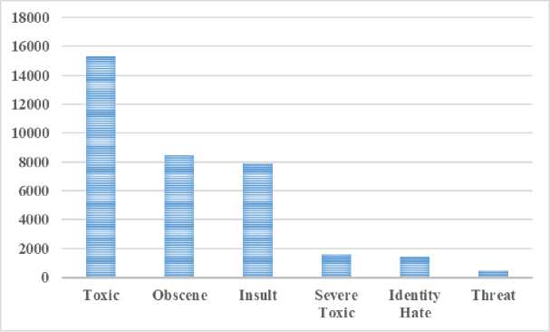
Fig.1. Distribution of types of toxic comments. change figure

Table 3. Toxicity comments distribution with overlap

Label	Toxic	ST	Ob	Th	In	IH
Toxic	100	10.43	51.82	2.94	48.02	8.51
ST	100	100	95.11	7.02	85.96	19.62
Ob	93.81	17.95	100	3.56	72.85	12.21
Th	93.93	23.43	62.97	100	64.23	20.50
In	93.23	17.41	78.14	3.90	100	14.73
IH	92.67	22.28	73.45	6.98	82.56	100

The accuracy of 15 classifiers combined with four feature encoding techniques are plotted in Table 4 and depicted in “Fig. 2.”. The combination of four feature encodings with word level n-grams, character level n-grams and character word bound generates twelve results for each prediction classifier. Thus, 15 multiply twelve i.e., 180 (15x12) results are used to investigate the classification performance. In the following tables, the word, char and cw represent word level ngrams, character level n-grams and character word bound respectively.

Table 4. Accuracy of different methods

Sl.	Classifier	BoW			TF-IDF			Hashing			CHI2
		word	char	cw	word	char	cw	word	char	cw	word	char	cw
1.	LR	0.879	0.897	0.896	0.898	0.898	0.899	0.899	0.884	0.884	0.903	0.903	0.903
2.	MNB	0.874	0.848	0.847	0.903	0.889	0.890	0.901	0.902	0.902	0.902	0.902	0.902
3.	BNB	0.879	0.773	0.773	0.902	0.530	0.530	0.900	0.901	0.902	0.902	0.902	0.902
4.	CNB	0.822	0.671	0.667	0.897	0.857	0.865	0.884	0.902	0.902	0.893	0.893	0.893
5.	Ridge	0.893	0.902	0.902	0.905	0.905	0.904	0.897	0.900	0.900	0.904	0.904	0.904
6.	SVC	0.903	0.901	0.901	0.902	0.902	0.902	0.902	0.902	0.902	0.904	0.904	0.904
7.	LSVC	0.853	0.781	0.575	0.879	0.899	0.900	0.885	0.892	0.893	0.903	0.903	0.903
8.	PA	0.841	0.881	0.884	0.866	0.769	0.753	0.864	0.878	0.879	0.030	0.030	0.030
9.	SGD	0.895	0.825	0.824	0.903	0.904	0.903	0.907	0.902	0.902	0.904	0.904	0.904
10.	KNN	0.895	0.874	0.874	0.903	0.882	0.880	0.903	0.872	0.869	0.901	0.901	0.901
11.	DT	0.899	0.899	0.899	0.900	0.899	0.901	0.900	0.901	0.899	0.904	0.904	0.904
12.	RF	0.902	0.902	0.902	0.902	0.902	0.902	0.902	0.902	0.902	0.904	0.904	0.904
13.	Bagging	0.899	0.900	0.900	0.897	0.906	0.906	0.898	0.901	0.901	0.903	0.903	0.903
14.	GB	0.879	0.897	0.897	0.878	0.868	0.864	0.879	0.860	0.877	0.898	0.898	0.898
15.	AdaBoost	0.890	0.900	0.900	0.880	0.889	0.889	0.885	0.888	0.888	0.902	0.902	0.902
Average		0.880	0.857	0.843	0.894	0.860	0.859	0.894	0.892	0.893	0.844	0.844	0.844

As stated in Table 4, the algorithms show good accuracy for all the feature encoding techniques except PA model with CHI2. Except CHI2 with PA, the lower and upper bound of accuracy of encoding schemes is 0.530 (char and cw)

and 0.907 (word) respectively. The CHI2 scored only 0.03 for the PA model; below the average level and needed more investigation. On the contrary, the outcome of CHI2 is positioned highest for eight algorithms. The BoW, TF-IDF and Hashing positioned top for one, three and four times respectively. Except CHI2, the word, char and cw options show the highest score for four, two and three times respectively.

Out of word, char and cw options the average lowest value is 0.843 achieved by cw of BoW. In contrast, the highest average value is 0.894 achieved by word option of TF-IDF and Hashing. Among BoW, TF-IDF, Hashing and CHI2 the top average (among word, char and cw) score is 0.893 generated by Hashing. The highlighted cells indicate best results of each row. Where nine classifiers show multiple best results specifically for CHI2, others show single best result. Considering all the results, the Hashing with word scheme outperformed using SGD classifier.

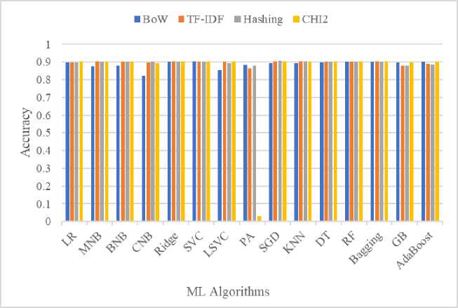
Fig.2. Max accuracy of vectorizers

The “Fig. 2.” is drawn by picking maximum accuracy of each vectorizer for individual classifiers. Where scores range from 0.822 to 0.907 except PA with Hashing. Even though, most of the vectorization techniques show similar results (except fractional difference) for the considered ML algorithms, the Hashing with SGD secured top position by scoring 0.907.

Besides accuracy comparison of different feature schemes, the ROC-AUC scores have been compared in Table 5 and depicted in “Fig. 3.”. Where, CHI2 shows low performance for eleven classifiers out of 15. On the contrary, word level n-gram reports highest roc-auc score for twelve times over the experimentation. Both the char and cw feature schemes show the highest score only for two times out of the results.

Table 5. ROC-AUC scores

Sl.	Classifier	BoW			TF-IDF			Hashing			CHI2
		word	char	cw	word	char	cw	word	char	cw	word	char	cw
1.	LR	0.937	0.779	0.780	0.973	0.934	0.929	0.972	0.829	0.830	0.656	0.656	0.656
2.	MNB	0.873	0.810	0.811	0.814	0.841	0.847	0.814	0.674	0.704	0.508	0.508	0.508
3.	BNB	0.907	0.670	0.698	0.704	0.735	0.736	0.827	0.665	0.664	0.656	0.656	0.656
4.	CNB	0.873	0.810	0.811	0.814	0.841	0.847	0.814	0.674	0.704	0.508	0.508	0.508
5.	Ridge	0.850	0.818	0.818	0.961	0.929	0.927	0.961	0.826	0.828	0.656	0.656	0.656
6.	SVC	0.936	0.752	0.746	0.860	0.889	0.876	0.940	0.822	0.827	0.626	0.626	0.626
7.	LSVC	0.926	0.795	0.729	0.971	0.932	0.930	0.965	0.832	0.833	0.656	0.656	0.656
8.	PA	0.907	0.744	0.744	0.960	0.921	0.923	0.947	0.810	0.822	0.600	0.600	0.600
9.	SGD	0.834	0.717	0.708	0.965	0.825	0.817	0.960	0.749	0.760	0.519	0.519	0.519
10.	KNN	0.730	0.617	0.617	0.548	0.728	0.732	0.633	0.642	0.644	0.603	0.603	0.603
11.	DT	0.721	0.675	0.675	0.714	0.732	0.730	0.702	0.731	0.724	0.650	0.650	0.650
12.	RF	0.774	0.700	0.700	0.632	0.830	0.825	0.762	0.717	0.717	0.655	0.655	0.655
13.	Bagging	0.619	0.502	0.504	0.726	0.656	0.630	0.737	0.529	0.519	0.573	0.573	0.573
14.	GB	0.531	0.619	0.619	0.588	0.431	0.435	0.588	0.626	0.690	0.443	0.443	0.443
15.	AdaBoost	0.939	0.820	0.820	0.945	0.922	0.920	0.943	0.837	0.837	0.651	0.651	0.651
Average		0.824	0.722	0.719	0.812	0.810	0.807	0.838	0.731	0.740	0.597	0.597	0.597

Among the plotted results, TF-IDF (char) with GB achieved 0.431 score; the lowest roc-auc score among the experimented models. Where, TF-IDF (word) combined with LR show highest score reporting 0.973. Out of twelve feature extraction options, the min and max average score is reported as 0.597 and 0.838 for CHI2 and Hashing (word) techniques respectively. In addition, out of four featuring options, the top average (among word, char, cw) score is obtained by TF-IDF i.e., 0.809.

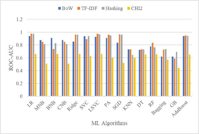
Fig.3. Max ROC-AUC of vectorizers

It is visible in “Fig. 3.” that the CHI2 records poor performance for considered ML algorithms. The BoW and Hashing report lower ROC-AUC for KNN, DT, RF, Bagging and GB. On the other hand, the bar of TF-IDF is above 80% except KNN, DT, Bagging and GB. However, the TF-IDF with LR model secured the highest score securing 0.973 for toxic comment classification in terms of ROC-AUC score.

RQ3: Which ML algorithm group is preferred to work on toxic comment classification?

To answer this RQ, the classifiers have been grouped as stated in Table 6 based on their application in this research.

Table 6. Average accuracy and ROC-AUC

Group	Classifiers	Accuracy	ROC-AUC
Regression	LR, Ridge, PA	0.813	0.817
Bayesian	BNB, MNB, CNB	0.894	0.754
Instance-based	SVC, LSVC, KNN, SGD	0.853	0.727
Decision Tree	DT	0.796	0.740
Ensemble	RF, Bagging, GB, AdaBoost	0.898	0.761

The average accuracy and roc-auc is calculated based on the formed groups. The ensemble group shows highest accuracy score i.e., 0.989. On the opposite, the regression group obtained 0.817 roc-auc; the highest among the groups. Even though, ensemble group illustrates maximum score for accuracy, the regression group shows more than 81% for both accuracy and roc-auc metrics. In addition, the accuracy of the regression group is decreased for the performance PA classifier. We observed that Regression group algorithms performed better than any other individual group.

RQ4: Which ML algorithm outperforms for classifying toxic comments in online behaviors?

In order to answer this RQ, the average accuracy and roc-auc scores of ML algorithms for twelve feature encoding strategies have been demonstrated in “Fig. 4.”. The ML algorithms show 0.642 or higher as accuracy rate for all the cases. Where the average accuracy range falls between 0.642 and 0.903, produced by PA and RF classifiers respectively.

On the other hand, the worst performance is shown by GB and Bagging in case of roc-auc metrics. Also, the KNN and DT records lower score. The seven classifiers scored between 70 to below 80. However, the LR, Ridge, LSVC and AdaBoost recorded 0.828, 0.803, 0.823 and 0.828 respectively. That is, all four classifiers show more than 80% roc-auc i.e., those are very close performer for classifying toxic comments in online behaviours. However, considering both accuracy and roc-auc, the best performers are LR and AdaBoost. The average accuracy of LR and AdaBoost is 0.895 and 0.893 respectively, where both of them achieved the same ROC-AUC i.e., 0.828.

■ Accuracy «ROC-AUC

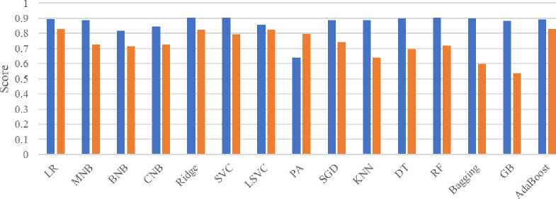
ML Algorithms

Fig.4. Average accuracy and ROC-AUC scores

As discussed, roc-auc scores, the CHI2 (word, char and cw) features generate lower and same result for maximum considered prediction algorithms. In addition, CHI2 records 0.03 as accuracy for PA classifier. Which indicate more experimentation with fine hyper-parameter tuning is needed to ensure that it performs same for word, char and cw level textual vectorization.

According to the results analysis, the BoW, TF-IDF and Hashing vectorization techniques are suitable for the toxic comment analysis domain. On the other hand, LR and Adaboost are the best performing algorithms for toxicity classification. Therefore, it is concluded that the LR and Adaboost can be combined with BoW, TF-IDF or Hashing feature extraction techniques for toxic comment analysis tasks.

5.    Conclusions

This paper demonstrated 15 supervised ML algorithms with four feature encoding schemes to explore the best combination model for toxic comment classification. Furthermore, to explore the best practices, n-gram word, n-gram character, and character word bound options have been applied with the vectorization techniques. The highest average accuracy is 0.894, achieved by the word option of TF-IDF and Hashing. For individual feature sets, the Hashing (word) with SGD and TF-IDF (word) with LR combination scored top for accuracy and roc-auc, respectively. However, considering average accuracy and roc-auc, the best ML algorithms are LR and AdaBoost for toxicity classification. The average accuracy of LR and AdaBoost is 0.895 and 0.893, respectively, where both of them achieved the same roc-auc, i.e. 0.828. According to the analysis of the results, the BoW, TF-IDF, and Hashing vectorization techniques are suitable for the toxic comment analysis domain. Therefore, it is concluded that the LR and Adaboost classifiers combined with anyone, i.e., BoW, TF-IDF, or Hashing method, can perform efficiently for toxic comment classification. In future, this research can be extended by investigating other prominent approaches like BERT[34], GRU and CNN [35] to explore the best combination for toxic comment classification.