Image Denoising using Tri Nonlinear and Nearest Neighbor Interpolation with Wavelet Transform

Published Online August 2012 in MECS

• I.    Introduction to Interpolation

In the mathematical subfield of numerical analysis, interpolation is a method of constructing new data points from a discrete set of known data points. In engineering and science one often has a number of data points, as obtained by sampling or experiment, and tries to construct a function which closely fits those data points. This is called curve fitting or regression analysis. Interpolation is a specific case of curve fitting, in which the function must go exactly through the data points. A different problem which is closely related to interpolation is the approximation of a complicated function by a simple function. Interpolation is way through which images are enlarged. Digital image interpolation is the recovery of a continuous intensity surface from discrete image data samples. It is a link between the discrete world and the continuous one. In general, almost every geometric transformation requires interpolation to be performed on an image, e.g. translating, rotating, scaling,  warping or  other applications. Such operations  are basic to any commercial digital image processing software. There are several issues which affect the perceived quality of the interpolated images: sharpness of edges, freedom from artifacts and reconstruction of high frequency details. We also seek computational efficiency, both in time and in memory. Classical techniques, such as pixel replication, bilinear or bi-cubic interpolation have the problem of blurred edges or artifacts around edges. Although these methods preserve the low frequency content of the sample image, they are not able to recover the high frequencies which provide a picture with visual sharpness [1].

Standard interpolation methods are often based on attempts to generate continuous data from a set of discrete data samples through an interpolation function. These methods attempt to improve the ultimate appearance of re-sampled images and minimize the visual defects arising from the inevitable resampling error [1].

Yohei Katsuyama and Kaoru Arakawa suggest interpolation techniques cause less blur than median type filter, if the noisy pixel is correctly detected. However, if the noisy pixel is falsely detected, the performance get largely degraded, since the output of weighted sum type filters gets more influenced by large amplitude impulsive noise than median type filtering [2]. Parker et al. pointed out that, at the expense of some increase in computing time, the quality of resample images can be improved using cubic interpolation when compared to nearest neighbor, linear, or Bspline interpolation. However, to avoid further perpetuation of misconceptions, which have appeared repeatedly in the literature, it might be better to refer to their Bspline technique as Bspline approximation instead of interpolation. Maeland named the correct (natural) spline interpolation as Bspline interpolation and found this technique to be superior to cubic interpolation [3] [4]. In more recent reports, not only hardware implementations for linear interpolation and fast algorithms for Bspline interpolation or special geometric transforms, but also nonlinear and adaptive algorithms for image zooming with perceptual edge enhancement have been published. However, smoothing effects are most bothersome if large magnifications are required.

• II.    Interpolation Methods

There are a variety of possible interpolation methods [5] [6] available when using geometric transforms in IDL. Interpolation methods include:

• A.    Nearest-neighbor interpolation: Assigns the value of the nearest pixel to the pixel in the output visualization. This is the fastest interpolation method but the resulting image may contain jagged edges.

• B.    Linear interpolation: Surveys the 2 closest pixels, drawing a line between them and designating a value along that line as the output pixel value.

• C.    Bilinear interpolation: Surveys the 4 closest pixels, creates a weighted average based on the nearness and brightness of the surveyed pixels and assigns that value to the pixel in the output image. Use cubic convolution if a higher degree of accuracy is needed. However, with still images, the difference between images interpolated with bilinear and cubic convolution methods is usually undetectable.

• D.    Tri-linear interpolation: Surveys the 8 nearest pixels occurring along the x, y, and z dimensions, creates a weighted average based on the nearness and brightness of the surveyed pixels and assigns that value to the pixel in the output image.

• E.    Cubic Convolution interpolation: Approximates a sync interpolation by using cubic polynomial waveforms instead of linear waveforms when re sampling a pixel. With a one dimension source, this method surveys 4 neighboring pixels. With a two dimension source, the method surveys 16 pixels. Interpolation of three dimension sources is not supported. This interpolation method results in the least amount of error, thus preserving the highest amount of fine detail in the output image. However, cubic interpolation requires more processing time.

• III.    Related work in Interpolation based Image denoising

Yasuhide Wakabayashi and Akira Taguchi propose a novel method for restoring impulsive noisy color images, which is constructed by the noise detector and the interpolator based on the demosaicing methodology [7]. Neil Toronto shows that edge inference achieves sharp, natural-looking interpolation by using neural networks to fit a sigmoid surface to every 3 x 3 block of samples in an image and combining the neural networks' outputs using Bicubic interpolation. Scaling every neural network's inputs by a constant multiplier changes the sharpness of the result. When noise is reintroduced, users of the algorithm have a sliding scale between Bicubic interpolation and edge inference of any sharpness [8]. Many interpolation methods already have been proposed in the literature, but all suffer from one or more artifacts. Linear interpolation methods deal with aliasing (e.g. jagged edges in the up scaling process), blurring and/or ringing effects [9]. Non linear or adaptive interpolation methods incorporate a priori knowledge about images. Dependent on this knowledge, the interpolation methods could be classified in different categories. The edge directed based techniques follow a philosophy that no interpolation across the edges in the image is allowed or that interpolation has to be performed along the edges. Robert G. Keys says that the cubic convolution interpolation function is more accurate than the nearest-neighbor algorithm or linear interpolation method. Although not as accurate as a cubic spline approximation, cubic convolution interpolation can be performed much more efficiently [10]. Shinfeng D. Lin derived a new technique for interpolating noisy frequency domain data is presented. This technique is generally based on rational function interpolation with least square-error method [11]. Often the interpolation is taken to be a linear combination of the input data and a given interpolation kernel. In order to analyze the quality of the interpolation method, Einar Maeland, study the very details of the (Fourier) spectrum, and the quality can then easily be attained. Since interpolation in reality is a problem of how to construct a low-pass filter, but need the details on the pass-band as well as the stop-band [12]. Hyeokho Choi demonstrated the efficacy of a new multistage maximum-smoothness interpolator for signal reconstruction and joint reconstruction / de-noising. His algorithm is straightforward, owing to the remarkably simple characterization of the Sobolev and Besove smoothness spaces by wavelets. In fact, for Sobolev space, the entire algorithm reduces to a simple least squares problem in the wavelet domain. Extension to higher dimensions (for image and volume data) is trivial [13]. Jenghwa Chang, analysis of a simply structured phantom shows that qualitatively good (i.e., few artifacts, size and shape of image peak nearly correct, sharp edge detection) images can be obtained and the rod can be accurately located using the constrained CGD method, when the reconstruction is based on noiseless detector readings and the matched weight matrix. The same data and reconstruction algorithm yielded unacceptable results when positivity constraints were not used. This strongly suggests that even if the use of constraints in reconstruction may lead to a nonlinear solution to a set of linear equations, the advantage confers by restricting the reconstructed results to a feasible and interpretable region more than compensates [14]. Jong Woo Han, proposed the novel interpolation method to handle the noisy input image. Since the bilateral filter effectively decomposes the input LR image into the detail and base layers, this method only deal with the noise in the detail layer. Jong Woo Han, empirically proved that the gradient energies in the corresponding region between the detail and base layers have the strong relationship. Therefore, depending on this relationship, it may be easy to distinguish texture information from the noise. The proposed method shows subjectively and objectively better performance to generate the sharp HR image from the LR image even when it contains the noise [15]. Guo Chao feng, used the piecewise cubic spline interpolation algorithm to de-noise image, the image obtains higher SNR Plus and smaller Mean Absolute Error [16]. The other important aspect of discrete geometric operations besides the transform is interpolation.

• IV.    Interpolation methodology

Interpolation is required as the transformed grid points of the input image in general no longer coincide with the grid points of the output image and vice versa. The basis of interpolation is the sampling theorem. This theorem states that the digital image completely represents the continuous image provided the sampling conditions are met. In short it means that each periodic structure that occurs in the image must be sampled at least twice per wavelength. From this basic fact it is easy at least in principle to devise a general framework for interpolation reconstruct the continuous image first and then perform a new sampling to the new grid points. This procedure only works as long as the new grid has equal or narrower grid spacing. If it is wider, aliasing will occur. In this case, the image must be pre-filtered before it is resampled. Although these procedures sound simple and straightforward, they are not at all. The problem is related to the fact that the reconstruction of the continuous image from the sampled image in practice is quite involved and can be performed only approximately. Thus, we need to consider how to optimize the interpolation given certain constraints. The ideal interpolation function in is separable. Therefore, interpolation can as easily be formulated for higher dimensional images. We can expect that all solutions to the interpolation problem will also be separable. Consequently, we need only discuss the 1-D interpolation problem. Once it is solved, we also have a solution for the n-dimensional interpolation problem [17]. We have proposes nonlinear tri interpolation for image de-noising in transformed domain as shown in figure 1. Wavelet transform is used for image denoising.

Input Noisy Image

----►

Apply Wavelet Transform

----►

Proposed Interpolation Model

-----►

Inverse Wavelet Transform

-----►

Output De-noisy Image

Fig. 1 Interpolation base Image de-noising

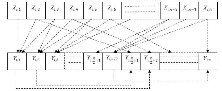
Fig. 2: Tri nonlinear Interpolation

• V.    Tri non Linear Interpolation

We have proposes a new tri non linear interpolation method for de-noising. It performs in two steps. Consider the X (i, j) is an input image, Y (i, j) is an output image for interpolation. In the first step, the row wise tri non linear interpolation perform by taking the average of three nearest variable which is the average coefficient of the image. After taking the average, detail coefficient is obtained by the taking the difference of average and the component of the image. By using row wise averaging and difference, image is split into two category, average and detail coefficient respectively. Average is low frequency component of the image and the detail is the high frequency component of the image. In the second step, column wise tri non linear interpolation performed by taking the average and the difference. This technique is suitable for image denoising as well as image enhancement. This technique will not add any blur in the obtained image. The tri non linear interpolation technique performed in the first step of row wise averaging as

X. ,1 + X ,2 + Xi ,3 = Y ,1

X ,3 + X ,4 + X ,5 = Y ,2

• X , n - 2 + X , n - 1 + X i , n = X i , n /2                   (1)

After taking the average, difference of the average and the image coefficient can be performed as

Y ,1 - X ,2 = Y , (. ^1

Y ,2 - X i ,4 = Y , ( n ) + 2

Y ,-- X.  = Y                            (2)

• i , n /2          i , n        i , n

This procedure is explained in the figure 2.

The tri nonlinear interpolation technique performed in the second step of column wise averaging as

X i, j + X 2, j + X 3,j = Y,j

^X 3, j ^{+ X} 4, j ^{+ X} 5, j = ^Y 2, j

^Xn - 2, j ^{+ X}n - 1, j ^{+ X}n , j = ^Xn /2, n                ⁽³⁾

After taking the average, difference of the average and the image coefficient row wise can be obtained from the average and original coefficient as

Y i ,1 - ^X i ,2 = D i ( n ) + 1

Y ,2 - X ,4 = D i ( n ^2

Y - X = D i,n/2         i,n          i,n

The column wise component can be obtained by taking the difference of the average and the image coefficient as

Y 1,j ^- X 2, J = D ( 2 b

Y ^2, j - ^X 4, j = D ( ⁿ ) + 2, j

Y „ . - X . = D .

n /2, j         n , j         n , j

(5-1)

After the interpolation we will get the average and detail coefficient. This coefficient will further undergo through our proposed mapping technique to reduce the noise at different level. We got the better result after inverse the same procedure. The inverse interpolation is required for modifying the noisy component to get the de-noisy image. The inverse interpolation performed in two steps. In first step, column wise interpolation of modified coefficient and in second step, row wise interpolation of modified coefficient. The inverse tri non linear interpolation procedure obtained from the modified row wise coefficient such as

^Y ,1 ^{+ Я} * ^Y i , ( 1 + ⁿ ) = Xi ,1

• ^Y ,1 - ² * ^Y i , ( 1 + ⁿ )= ^X i ,2

• ^Y ,2 - ^X* ^Y i , ( 2 + ⁿ )= ^Xi ,3

• ^Y i ,2 - ^Л* ^Y i , ( 2 + ⁿ )= ^Xi ,4

Y , _? + Л* Y.   = X.

i , n /2                i , n          i ,

¹ i , n /2    '^{L    J}i , n     i^i , i

(5-2)

The tri non linear inverse interpolation to obtain the column wise coefficient such as

• ^Y 1,J ^{+ X}* Y ( 1 + ⁿ ), j = ^X 1, J

^{Y      X}* ^Y ( 1 + 2 ) , j = X 2,j

• ^Y 2, j ^{+ X}* ^Y ( 2 + ⁿ ) , j = ^X 3, j

• ^Y 2, J - ^X* ^Y ( 2 + 2 ), j = ^X 4, J

Y и +A*Y =X . .

n /2, J ¹        ij , J     n-n - 1, J

Y — X * Y = X

Y n /2, j ^A Y n , j X j , j

We get the original coefficient after the interpolation technique.

• VI.    Interpolation nearest Neighbor

We have proposes nearest neighbor method for image de-noising in Wavelet domain. These techniques apply with wavelet transform to get de-noisy image from different noisy image. This nearest neighbor interpolation implementation model can be applied to the full image by moving this neighbor. After application of wavelet transform to noisy image we are getting average component. Average component consists of the noisy component at different levels. Nearest neighbor technique fill the component in between nearest average component. Filling the component will reduce the noise in the images. Consider the noisy image

Implementation of Interpolation: If the sequence of wavelet coefficient represented as

X1,,X2,X3,................,Xn-1,Xn(7)

After Nearest neighbor method, modified data can be expressed as

Modified data has Y component which is obtained by taking average of two near component i.e.

у    X 1 ⁺ X 2

Y1 =

Y    X 2 ⁺ X 3

Y2 =

Y - Xn - 1 + X n

Yn2

This modified coefficients fit in the window of image       modification of image data at that level.

as shown in figure 3. Figure 3 shows nearest neighbor

XI,1	XI,2	Х1,3	XI,4		XI,1	Yx< 1ДД2)	XI,2	■Х( 12 Д.31	XI,3	тхцздд)	XI,4
X2,l	Х2,2	Х2,3	Х2,4		•Х(1Д2Д)		•Х(1222|	Yx_™.r	•Х(1323|	¥х_™«г	¥х|1Д2Д)
X3,l	Х3,2	Х3,3	Х3,4		Х2,1	Тх<2Д22)	Х2,2	•Х(2223|	Х2,3	УХ|2.32Д|	Х2,4
Х4,1	Х4,2	Х4,3	Х4,4		*Х(2ДЗД)	Yx_™,=r	'Х(2232|	Yx_™.r	'Х(2333|	¥х_™«г	¥х<2ДЗД|
					Х3,1	•Х<3,132|	Х3,2	'хр233|	хз,з	• Х( 1,1:121	Х3,4
					¥х(ЗДДД|	Тх_™,=г	•Х(3242|	Yx_™.r	•Х(3.343|	¥х_™.«г	¥х,зддд|
					Х4,1	'Х(4ДД2|	Х4,2	•х(42ДЗ)	Х4,3	•Х(43>М)	Х4,4

Fig 3: Interpolation nearest Neighbor Technique

• VII.    Discrete Wavelet Transform

Wavelets are functions generated from one single function by dilations and translations [12], where dilation means scaling the wavelet and translation means shifting the wavelet. The wavelet expansion set is not unique. A wavelet system is a set of building blocks to construct or represents a signal or function. It is a two dimensional expansion set, usually a basis, for some class one or higher dimensional signals.

The wavelet can be represented by a weighted sum of shifted scaling function ϕ (2 t ) as,

ψ(t) = ∑h1(n)у/2ϕ(2t - n),      n ∈ Z (10)

n

For some set of coefficient h ₁ (n), this function gives the prototype or mother wavelet ψ ( t ) for a class of expansion function of the form

ψj,k(t)=2j/2ψ(2jt-k)                     (11)

w here 2 ^j the scaling of is t , 2 ^{- j} k is the translation in t , and 2 ^{j /2} maintains the L ² norms of the wavelet at different scales. The construction of wavelet using set of scaling function ϕ ( t ) and ψ ( t ) that could span all of L ² ( R ) , therefore function g ( t ) ∈ L ² ( R ) can be written as

∞ ∞∞

g(t) = ∑c(k)ϕk(t) + ∑ ∑d(j,k)ψj,k(t) (12)

k =-∞ j = 0 k =-∞

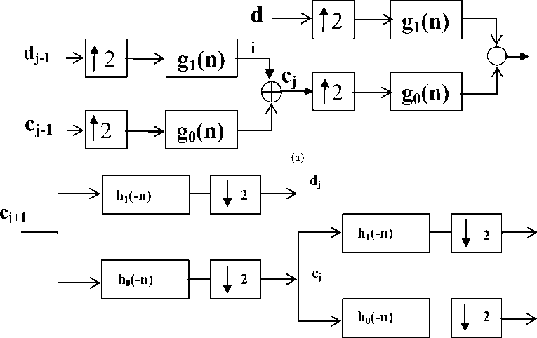
First summation in above equation gives a function that is low resolution of g ( t ) , for each increasing index j in the second summation, a higher resolution function is added which gives increasing details. The function d ( j , k ) indicates the differences between the translation index k , and the scale parameter j . Figure 4 shows the structure of two stages down sampling filter banks in terms of coefficients.

d j+1

(b)

Fig 4: a) Two stages up sampling Filter bank Figure b): Two stages down sampling filter

A reconstruction of the original fine scale coefficient of the signal made from a combination of the scaling function and wavelet coefficient at a course resolution which is derived by considering a signal in the j+1 scaling function space f ( t ) e Vj₊₁ . Figure 4 shows the structure of two stages up sampling filter banks in terms of coefficients i.e. synthesis from coarse scale to fine scale [5] [6] [7].

The DWT is identical to a hierarchical sub band system where the sub bands are logarithmically spaced in frequency and represent octave-band decomposition. By applying DWT, the image is actually divided i.e. decomposed into four sub bands and critically sub sampled as shown in Figure 5. These four sub bands arise from separable applications of vertical and horizontal analysis filters for wavelet decomposition as shown in Figure 5 [13]. The filters h0 and h1 shown in Figure 4 are one-dimensional Low Pass Filter (LPF) and High Pass Filter (HPF), respectively. Thus, decomposition provides sub bands corresponding to different resolution levels and orientation.

L

H

(a): Row wise decomposition

LL	HL
LH	HH

(b) One dimensional decomposition

Fig 5: Two-dimensional wavelet transform

LL	LH	HL
LH	HH
LH		HH

(c) Two dimensional decomposition

These sub bands labeled LH, HL and HH represent the finest scale wavelet coefficients, i.e. detail images while the sub band LL corresponds to coarse level coefficients, i.e. approximation image. To obtain the next coarse level of wavelet coefficients, the sub band LL alone is further decomposed and critically sampled using similar filter bank shown in Figure 4. This results in two-level wavelet decomposition as shown in Figure 5 [11]. The decomposed image can be reconstructed using a reconstruction (i.e. Inverse DWT) or synthesis filter as shown in figure 4. Here, the filters g1 and go represents low pass and high pass reconstruction filters respectively.

• VIII.    Implementation and Results

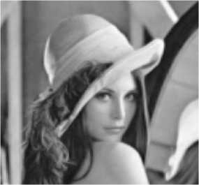
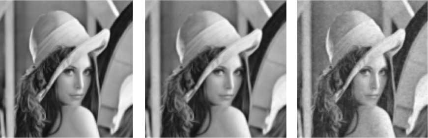
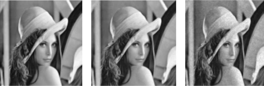
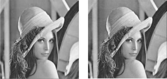
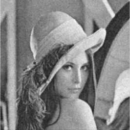
We have applied proposed technique to the ten images. As per the convenience we have shown the result for the Lena image. Add different noise to the Lena image. Then apply Wavelet Transform to the noisy image. We will get different sub band images at various level of wavelet decomposition. Every sub band will be further processed by applying the Tri non linear Interpolation methods. Each sub band will be up sampled by inverse Wavelet Transform. The transformed image has preserved the edges and original information. The next methodology we have used is the nearest neighbor interpolation for removing noise from the degraded image. The degraded image has gone through the Wavelet Transform. The Wavelet Transformed image it has approximation and detail coefficient. The nearest neighbor interpolation technique applied to the approximation coefficients. This different interpolated technique output chart in Wavelet domain as shown in figure 6. Results of Tri nonlinear interpolation technique in wavelet de-noising at different noise density are shown in figure 7. Results of nearest neighbor interpolation technique in wavelet de-noising at different noise density are shown in figure 8. All methods and there output PSNR at different noise density as shown in Table 1. This proposed technique has better PSNR as compared to existing technique. When noise density is increases then our methods has good quality images.

Table 1: Interpolation technique and there PSNR with Lena image

Result for Lena Grayscale image PSNR
Methods / Different Noise with different Variance	Gaussian Noisy Image			Salt and Pepper Noisy Image			Speckle Noisy Image			Poisson’s Noisy
	varianc e 0.0001	varianc e 0.001	varianc e 0.01	noise density 0.0005	Noise density 0.005	noise density 0.05	varianc e 0.0004	varianc e 0.004	varianc e 0.04
Interpolation Nearest Neighbor	13.1576	13.1027	12.6290	13.1604	13.1018	12.5764	13.1514	13.1122	12.6696	13.0717
Interpolation Nearest Neighbor with Wavelet	26.5744	26.4582	25.4196	26.5711	26.4005	24.8839	26.5738	26.4432	25.3757	26.3325
Tri Non Linear Interpolation with Wavelet	20.2815	20.1279	18.9282	20.2863	20.2289	19.1806	20.2806	20.1154	18.7866	19.9784
Tri Non Linear Interpolation Without Wavelet	25.8102	25.6505	24.3775	25.8135	25.6488	23.9458	25.8056	25.6362	24.2913	25.5017

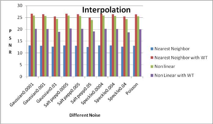
Fig 6: Interpolation methods in wavelet domain and there noise with different density

Fig 7 (a) Poisson

Fig 8 (a) Poisson

Gaussian noise 0.0001

Gaussian noise 0.001

Gaussian noise 0.01

Salt pepp 0.0005                            Salt pepp 0.005                            Salt pepp 0.05

Speckle0.0004                           Speckle0.004                            Speckle0.04

Fig 7 (b)

Fig 7: Different noise density output of Tri Non Linear interpolation methods

Gaussian noise 0.0001                     Gaussian noise 0.001

Gaussian noise 0.01

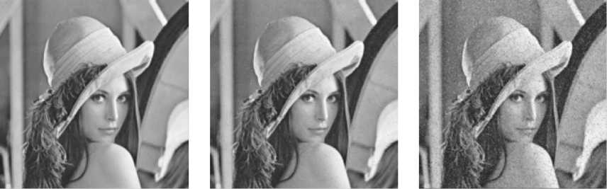
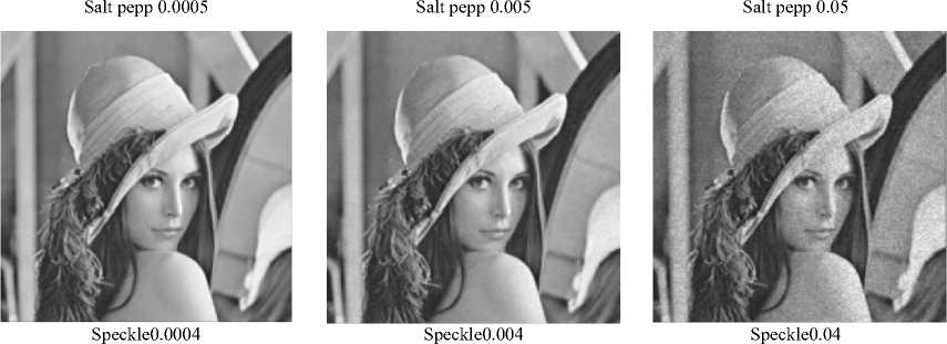
Fig 8 (b)

Fig 8: Different noise density output of nearest neighbor interpolation methods

• IX.    Conclusion

In this paper new methods nearest neighbor interpolation and Tri non linear interpolation is used for image denoising in wavelet domain. In contrast with existing methods our proposed scheme preserve the image detail at different noise density. The tri non linear interpolation scheme gives better PSNR as compared to the existing methods. Nearest neighbor interpolation technique has comparable good result. These methods do not introduce any blur in edges. These interpolation techniques applicable to all type of noise with different noise densities. If the noise density is increases nearest neighbor interpolation technique perform better as compared to the nearest neighbor.