Impact of weighting factor on cosine similarity based avalanche forecasting model

Published Online April 2019 in MECS

Snow avalanche is a constant threat for the human civilizations that reside in the hilly and mountainous regions. It is a natural process where gravity driven masses of snow tend to slide down mountain slopes in a rapid manner[1,2]. Along with snow, an avalanche also contains rock, soil, vegetation or ice[3]. An avalanche is broadly divided into three parts namely, the starting zone, the track of the avalanche and the run out zone. The word avalanche encompasses the complete process i.e. from the initiation of the avalanche in the starting zone, the route traced by the avalanche and the deposition in the run out zone[2]. An avalanche encompasses anything that comes in its path and hence it is the most lethal hazard occurring in the mountainous terrain.

An avalanche mainly occurs when there is a weakening in the snowpack. This usually happens when the gravitational force exerted on the top of the snowpack exceeds the binding force holding the snow together. The stability of the snow is dependent on fixed factors like slope, roughness, shape of the start zone and orientation to the sun. It is also dependent on the varying factors like amount of new snow, wind, water content and snowpack structure[4]. As a result, all these factors play an important role in forecasting of snow avalanche.

Avalanche forecasting is defined as predicting snowpack instability in space and time relative to a given triggering level[5]. The data that is required for forecasting of an avalanche is mainly classified into three classes. This classification is based on the ease of interpretation and the relevance of the data to avalanche prediction. It is given as follows:

Class I: Stability factors.

Class II: Snowpack factor.

Class III: Snow and weather data.

According to these classes, a lower class number depicts high certainty and relevancy with respect to avalanche prediction. Stability factors depict the results of the stability test that provide avalanche occurrence information for a particular region. Snowpack factors provide information about the internal structure of the snowpack. Snow and weather data is numerical data which is measured near or above the snow surface. In this paper class III data is used for avalanche forecasting. Use of statistical methods for forecasting an avalanche has formed an important aspect of avalanche forecasting. A brief review of the forecasting methods for snow avalanche is presented in the section II. On the basis of the review of the existing methodology, it was observed that euclidean distance is used mostly as a distance metric to calculate the distance. Use of Mahalanobis distance and cosine similarity is also observed for calculating the distance between the neighbours[6,7]. Present work explores the application of the weighting factors to the significant parameters to the nearest neighbour based avalanche forecasting model using cosine similarity.

The remainder of the paper is organised as follows: Section II provides information about the related work. Section III describes the proposed work. Section IV provides information about the study area and the data that is used for the current work. Section V presents the results of the proposed work and section VI concludes the paper.

• II.    Related Work

A non-parametric approach involving the nearest neighbours of a particular day was suggested to find whether an avalanche can occur on a particular day[8]. This was done by calculating the conditional probability of a particular day given by (1).

Pr{Avalanche on day i} = nA. (1) N where, N is the total number of neighbours considered and nA is the total number of avalanche days amongst the neighbouring days. The nearest neighbour method(NXDAYS) was implemented by obtaining the distance(r) between the neighbouring days by (2).

r²= ∑ _iΔx i ². (2)

where, x is the value of the parameters between the considered days. Further the use of weighting factor was introduced that helped in providing importance to the significant parameters[9]. A need for daily avalanche report was also suggested. The performance of NXDAYS was reviewed after being operational for three years at Weissfluhjoch[10]. The critical level for differentiating an avalanche day was set to 0.3. This signified that a day would be considered as an avalanche day if 3 out of the 10 nearest neighbours are avalanche days. This model was further extended by taking into account earlier weather conditions along with the evolution of the snow cover[11]. The values for some variables were calculated by taking into consideration their behaviour for a particular period or previous days to avoid seasonal influence. This model was not only successful in finding similar periods along with similar days but also provided better forecast than the conventional model.

A new method employing parametric discriminant analysis using Bayesian statistics was used to find the probability of whether a data vector belonged to avalanche days or non-avalanche days based on the historical data[6]. The model also used nearest neighbour algorithm along with Mahalanobis distance as a distance metric instead of Euclidean distance. NXLOG 2.0 was implemented that used machine learning functions for improving the reliability in avalanche forecasting[12].

This was a combination of NXD that used the nearest neighbour model and AVALOG that used the artificial intelligence techniques. Future enhancement was to optimize the machine learning techniques so that model performance will improve by itself. NN3 was developed to forecast avalanche occurrence up to 24 hrs by using the data acquired by an automatic weather station[13]. The database used for the said work represented 3 hour periods. The total 22 parameters were obtained from the basic 4 parameters i.e. Temperature, Wind Speed, Wind direction and Precipitation and the concept of normalized distance was also explored.

An improved and further developed version of NXDAYS, NXD2000 was implemented that dealt with the functions giving importance to certain values of variables and explanatory variables[9,14]. Nearest neighbour algorithm was used for regional level avalanche forecasting for an area up to 5000km2[15]. The model was able to produce the official SLF avalanche forecast for 52% of the days but failed for periods where snow cover stability was important. Principal component analysis was used as a tool for data reduction and to obtain independent variables in a tool named Astral. This tool was further used to find ten analogous days by nearest neighbour approach[16]. The absence of internal variable of the snowpack was considered as an inefficiency of the tool. Another tool to overcome this inefficiency was put forth that integrated variables, which described the internal structure of the snowpack in the tool.

Though weighting of significant parameters played an important role in the earlier models, the process was manual. Automating weighting of parameters was put forth by the use of genetic algorithm in the model ‘Cornice’[17,18]. Cornice also supported batch testing and was developed in java and provided output in three modes. Cornice did not use elaborate variables yet the results were similar to NXD2000. Hence the model showed that genetic algorithm provided similar results even in absence of elaborate variables. Here the distance was measured for the day to be forecasted and three previous days from neighbours so as to find pattern of similar days as well along with the neighbours. Fitness measures were used to compare the working of the model.

A new probabilistic method for forecasting was proposed that combined Geographic Information System with modified meteorological nearest neighbour approach[19,20]. This proposed tool allowed to visually explore, at multiple scales, the regional spatial patterns of avalanche activity. It further allowed to investigate the relationship between weather parameters and spatial pattern of avalanche activity. A supplement to the avalanche forecasting method was suggested that only considered the parameters which fell in between a specific range with regards to the particular day and the neighbours were searched only in the boundary of +15 days from the forecasted day[21]. A criteria was also decided with regards to base range and the range constants, that incorporated the uneven effects of the parameters. This was done to lessen the effect of parameter’s critical changeovers on avalanching.

Mesoscale Weather forecast model(MM5), a weather parameter simulation model, was integrated with the nearest neighbour based avalanche forecasting model to predict avalanche occurrence situation for up to 4 days[22]. Based on the values provided by the MM5 model, the values for derived parameters were calculated and used in avalanche forecasting model. The preliminary results were encouraging despite low prediction accuracy for the second, third and fourth day. An attempt was made to use artificial neural network for avalanche forecasting for the Chowkibal-Tangdhar sector (CT Sector) of Kashmir, India[23]. Values for avalanche Probability (P av , P nav ) were calculated by taking into account the relative distance of the neighbours with regards to the forecasted point for both avalanche and non-avalanche days present in the neighbours. The overall performance of the model met the desired levels satisfactorily.

A nearest neighbour model was used that accepted hourly electronic weather sensor data to produce automated avalanche occurrence prediction for up to 12 hrs[24]. To handle the unavailability of the data due to sensor issues or missing values, filtering mechanism was developed. Identification of the significant factors in the formation of an avalanche is a very important aspect in the avalanche prediction scheme. Two feature ranking methods - Relief-F and Sequential Forward Generation were used to find the relative significance of the numerous snow and meteorological features that are supposed to be related with the Avalanche Occurrences[25]. Both methods showed notable output and this work could help in removing the subjectivity present in avalanche forecasting process. Artificial bee colony algorithm, was explored to attune eNN10,a nearest neighbour model developed in India for snow avalanche forecasting[26]. The objective function Heidke Skill Score(HSS) was used as a fitness matrix. The comparison of the HSS value after model calibration by ABC algorithm and without calibration by keeping all the decision variables to 1, showed a substantial gain in the output. However, the mean value of HSS observed was far from the ideal score of 1. Further to speed up the process of calibration of eNN10 by using ABC Algorithm, NVIDIA Tesla C2050 GPU governed by MATLAB-CUDA programming framework was used[27].

A new method was proposed that explored the use of cosine similarity with nearest neighbour implementation to find the avalanche occurrence situation[7]. The results of this method are encouraging however need for further tuning of the model is observed. Present work focusses on the application of weighting factor to the cosine similarity based nearest neighbour model in order to increase the accuracy of the model.

• III.    Proposed Work

An avalanche occurs due to change in values of different parameters. Hence it is necessary to consider all these factors for finding the avalanche occurrence probability. All the days in the dataset have values for the different parameters and an avalanche occurs only when certain values for parameters are witnessed. The notion behind this work is, if an avalanche had occurred for a particular set of weather condition, then it can occur again if alike conditions are observed. When nearest neighbour is applied on the dataset, the goal is to find the days having maximum similarity value with the present day. Days having the maximum similarity with the present day are considered as neighbours and depending on the avalanche situation for these ten days, it is decided whether an avalanche can occur on a particular day or not.

Cosine similarity has been considered more appropriate than euclidean distance, mahalanobis distance for textual as well as non-textual dataset[28]. In cosine similarity, the similarity between two vectors is given by (3) where A and B are the vectors and A i and B i are their components respectively. The cosine similarity of two identical vectors is one. Hence the vectors that are similar will exhibit high value for cosine similarity. Similarly, in avalanche forecasting the days that are similar to each other have high value of cosine similarity.

∑ ^{n AB}

Cosine Similarity =     i=1          .

nn ∑Ai2

i=1i=1

The preliminary results of using cosine similarity with nearest neighbour are encouraging. However, in order to improve the accuracy of the model, mechanism is required to give additional preference to important parameters. In case of unique situations when avalanche had occurred, a certain change is observed in some significant parameters. Proper handling of such situations is also needed. Additional preference to parameters has been previously provided by using the concept of weighting[9,25]. But for the previous work, euclidean distance was used as a distance metric. For the current work, concept of weighting has been applied along with cosine similarity. The formula to calculate the similarity in the current context is given by (4) where A and B are vectors with A i and B i as their components respectively and w is the weighting factor where w i is the weighting factor for each parameter. For the current work, the vectors A and B are the values of the parameters for the days whose similarity is to be found.

n ∑ w_iA_iB_i

Similarity between days =   i=1           .

nn ∑Ai2

i=1i=1

The steps for finding the avalanche forecast for a particular day using the concept of weighting are given as follows:

• 1.    The similarity between a particular day and the rest of the dataset is calculated using (4).

• 2.    The rest of the days from the dataset are arranged in the decreasing order of their similarity with the particular day i.e. higher the similarity, closer is the past day (day from the dataset) to the particular day.

• 3.    The nearest neighbours to the particular day are obtained by taking first 10 days from the order obtained in previous step.

• 4.    The avalanche occurrence situation for all the ten neighbours is found.

• 5.    Probability of avalanche occurrence is found out by (1).

• 6.    If the probability of avalanche occurrence is greater than or equal to threshold value, then the particular day is considered as an avalanche day.

The number of nearest neighbours that are considered for the proposed work are ten[11]. Further the value of threshold is considered as 0.3[10]. Hence if the number of the avalanche days is greater than or equal to three, the particular day (day whose forecast is to be found) is considered as an avalanche day.

• IV.    Study Area and Parameters of Interest

  The proposed model is implemented using the snow and meteorological data for the Bahang (32.2727° N, 77.1823° E) village of Himachal Pradesh, India. This village is located in the Pir Panjal range of the Lower Himalayan Zone[29]. Geographical Location of Bahang Village and its satellite map is given in Fig.1. Snow and meteorological data used for the current work is obtained from the observation station installed at Bahang (2192 m above sea level)[30]. From all the parameters that are obtained from this observation station, 9 parameters are selected for the current work based on their effect on avalanche occurrence. The data for all these parameters is obtained daily at 0830 hrs and 1730 hrs (both IST (GMT + 5.30)) for the months of January, February and March from the year 2005 to 2013. Though this data is collected daily at the observation station, sometimes due to some glitch, values of some parameters are not acquired. The missing values are handled in the current work by recalculating them by using the relation between wet temperature, humidity and dry temperature[31].

The whole dataset i.e. from Jan 2005 to March 2013 is divided into 2 parts i.e. Training Dataset and Testing Dataset for the current work. Two different combinations of training and testing dataset are used for experimental work. These variations help us to understand the working and the correctness of the model in different combinations. The combinations of the datasets used for the current study are given in Table 1.

Table 1. Dataset combinations

Dataset Combination No.	Training Dataset	Testing Dataset
I	Jan 2005 to March 2011	Jan 2012 to March 2013
II	Jan 2005 to March 2012	Jan 2013 to March 2013

The contribution of weighting factor has a significant impact on the accuracy of the model. Amongst the parameters that are selected for the model, some parameters have a higher significance because of their effect on avalanche occurrence. For instance, the amount of snowfall in a short duration is of more importance than same amount of snowfall in a comparatively longer duration. The weighting factor for the parameters having higher significance is 1 and for the rest of the parameters in 0.5. The list of parameters along with their weighting factors that are used for the current study are summarised in Table 2.

Table 2. List of parameters along with weighting factors

Sr. No	Variable	Unit	Weighting Factor
1	Wet temperature	°C	1
2	Average wind speed	kmph	0.5
3	Humidity	%	1
4	Amount of fresh snow	cm	1
5	Fresh snow water equivalent	mm	1
6	Height of snow	cm	0.5
7	Snow temperature	°C	0.5
8	Penetration of snow	cm	0.5
9	Rate of snow fall	cm/min	1

• V.    Results and Discussion

  The total dataset used for the proposed work consists of 812 days. Data recorded at 0830 hrs is used for the current work. An avalanche occurrence event is characterized as “Yes” event when an avalanche has taken place or “No” event when an avalanche has not taken place. To check the accuracy of the forecasting model and identify the correct predictions and error, the classical True/False confusion matrix is used[32]. The correct predictions are True Positives(a) and True Negatives(d) and the errors are False Positives(b) and False Negatives(c). These are summarised in Table 3. The True Positives are those events that have occurred as well as have been properly detected by the model. False Positives are those events that have not occurred but the model has forecasted them as “Yes” events. Similarly, False Negatives are those events that have occurred in real time but are forecasted as “No” events by the model. True Negatives are those events that have neither occurred nor forecasted as “Yes” by the model.

Table 3. Confusion matrix for binary events

Observed Forecasted	Yes	No
Yes	True Positive (a)	False positive (b)
No	False Negative (c)	True Negative (d)

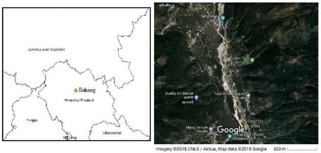
Fig.1. Geographical Location of Bahang Village in India and Satellite map of Bahang village

For the analysis of the model, change in the values of confusion matrix after the application of weighting factors for both the combinations of training and testing dataset is observed. Further, the accuracy of the model is also evaluated with the help of performance measures. The measures used for the current work are Critical Success Index(CSI) and Bias. Critical Success Index provides the ratio of correct forecasts to the total events observed and/or forecasted[33]. It is mainly useful in events where “Yes” event occurs less frequently than “No” events. It is given by (5).

Critical Success Index =    a a+b+c

.

Similarly, Bias is the measure of the tendency of the model to over forecast or under forecast. It is calculated as (6).

a+b

Bias = a+c

.

Table 4. Effect of weighting factors on values of confusion matrix (values are in %)

	Dataset Combination I	Dataset Combination II
Change in the value of a	0.0000	2.2222
Change in the value of b	-3.3149	1.1111
Change in the value of c	0.0000	-2.2222
Change in the value of d	3.3149	-1.1111

The change in the values for confusion matrix are summarised in Table 4. A positive number represents an increase in the value after application of weighting factor whereas a negative number depicts a decrease in the value after the application of weighting factor.

Similarly, the values for the performance measures for both the combinations of the dataset are summarised in Table 5.

• A.    Changes Reflected In Dataset Combination I

  There is no change in the value of True Positive(a) and False Negative(c). However, a decrease is observed in the value of False Positive(b). This indicates a reduction in the False Positives that are being provided by the model for Dataset Combination I after the application of weights. Hence the number of events that are wrongly forecasted as “Yes” events by the model are reduced after applying the weighting factor. Similarly, there is an increase in the value of True Negative(d), which means that values that were wrongly forecasted as “Yes” events have been corrected after the application of weights. The values of the performance measures are also encouraging. The value of Bias has reduced from 4.33 to 2.33. This means the even though the model is over forecasting, there is definitely a decrease in the model’s tendency to over forecast. The best possible value for CSI is one[33]. Hence, from the value of CSI, it can be seen that the model is improving with the application of weights. An increase of 0.1978 is observed in the value of CSI for dataset combination I.

• B.    Changes Reflected In Dataset Combination II

An increase is observed in the values of True Positive(a) after application of weights. This is good as there is an increase in the number of the correctly “Yes” forecasted events. However, there is also an increase in the value of False Positive(b). This means that the model is also forecasting some events as “Yes” which are actually “No” after applying weights. Further there has been a decrease in the value of False Negative(c). This is considered as good as there is a decrease in number of instances which are actually “Yes” events but were predicted as “No” events. Lastly, a decrease is observed in the value of True Negative(d). This is not good as some values have been forecasted as “Yes” which are actually “No” events.

Table 5. Values for Performance measures

	Dataset combination I		Dataset combination II
	Without weights	With weights	Without weights	With weights
Bias	4.3333	2.3333	0.3333	1.3333
Critical Success Index	0.2308	0.4286	0.3333	0.7500

The value of Bias signifies that the model was under forecasting without the application of weights. However, after application of weights, the model tends to over forecast. The value of Bias for an unbiased forecast is one[33]. Hence, it is observed that even though the model is over forecasting, the value of Bias is tilting more towards 1 after the application of weights. Similarly, there is also an increase in the value of CSI by 0.4167 after application of weights which shows good performance of the model after applying weights.

Hence, the application of weighting factor seems to have a positive effect for the Dataset Combination I. In case of dataset combination II, the effect is not completely positive. Though there is an increase in the correctly forecasted “Yes” event, a small rise is also observed in the value of False Positives. The values of performance measures depict an improvement in the model after application of weights for both the dataset combinations.

• VI. Conclusion

  Accurate forecast of snow avalanche is the need for wellbeing of mankind. The use of cosine similarity with nearest neighbour for snow avalanche forecasting has been encouraging. The proposed work explored the application of the weighting factors to the significant parameter with an aim to increase the accuracy of the model. The values for the weighting factors are decided based on the effect of each parameter on avalanche occurrence. The impact of application of weighting factor is reflected in the values of confusion matrix and the performance measures. The results of proposed model are promising. A positive effect is observed for dataset combination I. For dataset combination II, though increase in True positive is observed, increase in the False Positive(b) is also seen. Similarly, an increase of 0.1978 and 0.4167 is observed in the value of Critical Success Index for dataset combination I and II respectively. In case of Bias, the model tends to over forecast for both the dataset combinations.

Acknowledgement

The Authors are thankful to Director, SASE (Snow Avalanche Study Establishment) for providing us with the snow and meteorological data for Bahang, Himachal Pradesh for our research study purpose.