Implementation of Carlson based fractional differentiators in control of fractional order plants

Published Online September 2018 in MECS

The fractional order differentiation and integration in mathematics is an old topic, dated back to seventeenth century, but could not be used in many applications because of the complexity associated with it. In recent years researches have been able to explore many potential applications of fractional calculus in science, engineering and management / business administration particularly in physical chemistry [1, 2], biomedical engineering [3], control system [4-7], signal processing [8] and inventory management [9]. Fractional differentiators and integrators are an integral part of fractional filter based signal processing and fractional feedback control of complex systems and chaotic systems [10]. A fractional order system is an infinite dimensional filter having irrational continuous time transfer function in the s-domain. The need to study the rational approximation of fractional order systems is mainly because the hardware realization of fractional order systems is a difficult task. The fractional order systems are usually approximated by a finite order rational transfer function. There are a few well known approaches viz. Carlson method [11], Matsuda method [12], Charef method [13], Oustaloup method [14] and method proposed by Xue et al. [15] to obtain the rational approximation. Out of these, some methods yield very high order integer order models for attaining desired accuracy. However, the realization, implementation and simulation of higher order models is often not feasible. This necessitates reducing the order of the model, either by simplifying the model or computing a lower order model, while preserving the necessary properties and characteristics of the original integer order model obtained. This requires treating the original model mathematically with numerical linear algebra and also using iterative solution techniques for linear systems. There are some model reduction methods viz. Pade approximation method, Pade-via-Lancoz (PVL) method [16], truncation methods [17], sub-optimum H2 pseudo-rational method [18], Asymptotic Waveform Evaluation [19], etc to name a few. Another method for model reduction is Proper Orthogonal Decomposition. This method can also be applied for solving non-linear partial differential equations. All the model order reduction methods available in literature aim to have a balance between solution accuracy and computational effort. As such, simplified models are a replacement of original complex models resulting in reduced computational complexity.

In this paper, Carlson method has been used to develop integer order models of fractional differentiators. Since this method is based on the Newton Iterative process, the order of the approximation obtained depends only on the fractional order α, and cannot be chosen a priori.

Moreover, the orders obtained are very high and are unrealizable in  their original form.  A generalized procedure adopted in such cases, is to reduce the order of the approximation obtained using  order  reduction techniques. We  have used three  order  reduction techniques, namely, Balanced truncation method, Matched DC gain method and Pade approximation method and have derived lower order models of fractional differentiators, making them easily realizable. Simulations are performed and a comparison of the responses of these models with the original response is presented. In order to accentuate the validity of the proposed work, fractional order plant has been controlled using fractional PD and fractional PID controller, and results investigated. The responses of these closed loop systems are observed to outperform the results shown in [15]. In [20] the authors used self-tuning PID controller for Permanent Magnet Synchronous Motor (PMSM) vector control and in [21] and [22], PI and PID controllers are discussed as control strategies for Permanent Magnet Synchronous Generator (PMSG) based wind energy conversion system and 3Φ Induction Motor (3ΦIM) speed control system respectively. In a similar manner, the fractional PD and fractional PID controller presented in this paper can be used as control strategies for the speed control of these machines.

The paper is organized as follows: Carlson method of approximation, the basis of various model order reduction techniques and the reduction methods used in this paper are discussed in Section 2. The performances of the proposed models of fractional differentiators are presented in Section 3. To show the effectiveness of the proposed models and that of the technique used for order reduction, illustrative examples with detailed analysis are presented in Section 4. Section 5 concludes the paper.

• II.    Realated Works

This section starts with describing the Carlson method of approximation and continues to discuss the application of model order reduction to the integer order models of fractional order systems. A brief description of three order reduction techniques are also presented.

• A.    Carlson Method

The fractional order system, F ( s ) in the s -domain is in the form

F ( s ) = s ^a ; aG R               (1)

where α is the fractional order.

The integer order approximation, F_i ( s ) of fractional order system using Carlson method is

F ( s ) = F - 1 ( s )

i g N (2)

In the first iteration i.e. for i=1 , F 0 ( s ) is chosen as 1 . Also, ( 1/α ) can take only integer values [11, 23], that is 1/α = ±2, ±3, ±4, ..…. .

In second iteration i=2, and substituting α = 0.1, the approximated integer order transfer function of one-tenth differentiator is s . =

'   1.494 s ¹² + 28.58 s ¹¹ + 197.2 s ¹⁰ + 744.3 s ⁹ + 1790 s ⁸ + 2944 s ⁷

+ 3426 s ⁶ + 2846 s ⁵ + 1669 s ⁴ + 666.1 s ³ + 167.7 s ² + 22.54 s + 1

s ¹² + 22.54 s ¹¹ + 167.7 s ¹⁰ + 666.1 s ⁹ + 1669 s ⁸ + 2846 s⁷

(+ 3426 s ⁶ + 2944 s ⁵ + 1790 s ⁴ + 744.3 s ³ + 197.2 s ² + 28.58 s + 1.494 J

Similarly, for α = 0.2 in (2), the approximated integer order transfer function of one-fifth differentiator becomes

( 2.25 s ⁷ + 29.77 s ⁶ + 107.4 s ⁵ + 185.6 s ⁴ + 175.1 s ³ + 88.8 s ² + 20.39 s + 1 ^

( s ⁷ + 20.39 s ⁶ + 88.8 s ⁵ + 175.1 s ⁴ + 185.6 s ³ + 107.4 s ² + 29.77 s + 2.25 J

Similar approach can be applied to all values of α (0 < α < 1) to obtain the approximated order integer transfer function of fractional differentiator [11, 23].

• B.    Model Order Reduction

The transfer function of a finite dimensional dynamical system in the Laplace domain is represented in the form

_F(. = Y ( s ) ₌ У + bm - 1 sm " 1 + .A

U ( s )    a_nsⁿ + а_п_^^{п - 1} + .... a₀

The state representation of such a system in the matrix form is

x Г A B1Г x = r n

y L c d JL u and in the equation form is

x = Ax + Bu

y = Cx + Du

where u is the input, y is the output, and x is the state variable.

The system equations in the Laplace domain are sX (s) = AX (s) + BU (s) Y (s) = CX (s) + DU (s)

The state equations in the transfer function form may be written as

F ( s ) = Ys ) = C ( si - A )^{- 1 B +} D        (9)

Some of the model order reduction methods available in literature are based on transfer function models and others on state space models [24, 25]. Model order reduction based on transfer function is equivalent to approximating the original model of order N to approximated model of order r, where r < N and for state space model, it is reducing the matrix A but B and C unchanged.

A good approximant should have small approximation error while preserving the necessary properties and characteristics of the original system and the reduction procedure should be cost effective and computationally efficient.

Most of the methods form their basis via one or more of the following mathematical processes. These mathematical processes are discussed below.

• 1)    Moments

Applying Taylor series expansion [16] to (5) about s = 0 the resulting expression is

F (s) = m0 + ms + m2s2 + where m0, m1, m2 … are the moments of the transfer function. The ith moment of the transfer function is

. to tl mi-=(-1)'f- f (t) dt

0 t !

where f(t) is the time domain expression of F(s). Similarly the ith moment of (9) at s = s0 is m,= C (s о I - A I B(12)

After calculating the moments, a model reduction technique, like the Pade approximation or Pade-via-Lancoz (PVL) method is applied to obtain a lower order approximation.

• 2)    Singular Value Decomposition

Singular Value Decomposition [26] is a decomposition of matrix A into matrices X, Y and S, where X and Y are unitary matrices and S = diag (σ1, … σn) and A=XSY*. The σi are the singular values of A, which are the square roots of the largest n eigen values of A*A or AA*. Hankel Singular Values are to model order what singular values are to matrix rank. Hankel Singular Values define the energy of each state in the system where as eigen values define a system stability. To obtain a simplified model, smaller energy states are discarded. By keeping large Hankel Singular Values most of the necessary system characteristics like stability and magnitude and phase responses are preserved.

For a stable state space model ah = 4^Q2)          (13)

where σ h is the Hankel Singular Values, P and Q are controllability and observability grammians satisfying the two Lyapunov equations.

AP + PA T + BB T = 0

A T Q + QA + C T C = 0

The error is measured in terms of peak gain across frequency (H∞ norm) and the error bounds are a function of the discarded Hankel Singular Values.

The additive error bound is

N

|| F - ^рД „< ² z ^h            (¹⁵)

r + 1

The multiplicative (relative) error bound

II F "’ ( F - F red !(1 + 2^. ('F+^h + ^h ))-1     ⁽¹⁶⁾

where F is the original model and F red is the reduced order model and σ h are the h^th Hankel Singular Value of the original model F . The model order reduction technique like Optimal Hankel Norm Reduction method is based on this mathematical process.

• 3)    Krylov subspaces

For a linear system Ax = B having n equations and n variables, a subspace spanned by a sequence of column vectors is known as Krylov subspaces [27].

For a symmetric matrix A and starting vector b, Right Krylov subspace is defined as к (A, b) = span {b, Ab, A2 b,......, An-1 b}        (17)

For a non-symmetric matrix A and starting vector b , Left Krylov subspace is defined as

к ( A T , c ) = span { c , A T c , ( A T ) c ,......, ( A T )    c }      (18)

Model order reduction techniques relying on Krylov subspaces involve some preconditioning for fast convergence of the iterative method and some orthogonalization schemes, such as Lancozs iteration for Hermitian matrices or Arnoldi iteration for more general matrices.

The model order reduction technique like Arnoldi and PRIMA method, Laguerre method is based on this mathematical process.

• C.    Reduction Methods

The three order reduction methods used in this paper are briefly discussed here. These are:

• 1)    Balanced truncation method (method 1)

In this method for continuous state space model, first the Hankel singular values is found, as such respective energy of each state is known and the states to be eliminated are directly determined. The controllability and observability grammians are found. Then Schur balance truncation algorithm [28] is applied to obtain the reduced order model based on the states chosen to be eliminated. The additive error bound on the H∞ norm is taken as a measure of the transfer matrix and is a function of the discarded Hankel Singular Values.

• 2)    Matched DC gain method (method 2)

This method is based on Hankel Singular Value decomposition. For the state space model the state vector is divided as x = [ x ₁ ; x ₂], where x ₁, are the larger energy states, to be kept and x 2 , with smaller energy states, to be discarded.

x ₁

x ₂

y = [ Cx C2 ] x + Du x is made equal to zero and a reduced order model is obtained by solving for x1, given by x1 =[ A11  A12 A22 A21 ] x1 +[ B1  A12 A22 B2 ] u y == [C - C2A2-1 A! ]x + [D - C2A2-1 B2 ]u

The limitation of this method is that in continuous time A 22 should be invertible.

• 3)    Pade approximation method (method 3)

In this method, first the moments are calculated for the transfer function of the original higher order model. Then Pade approximation method is applied to obtain the reduced order model by matching the moments with the desired lower order model. The coefficient of each power of s is equated for the two sides to match.

• III.    Performance and Discussions

We have developed reduced order models of fractional differentiator s^α (0 < α < 1) using the three methods of order reduction discussed in section 2. The reduced models are all of order 3. All the models are listed in Table 1.

Figs. 1, 2 show the frequency responses of the original and reduced order models of fractional differentiator for α = 0.1, 0.2 respectively. In Fig.1 the response of onetenth differentiator using Carlson method (3) is compared with the response of the reduced 3^rd order models using the three methods. It is observed that the response of the model obtained using methods 1 and 2 match exactly with the response of the original model in the entire frequency range [10^-2, 10²] rad/sec for both magnitude and phase plots, where as the response of the model obtained using method 3 slightly deviates from the response of the original model in the frequency range [3, 40] rad/sec for the magnitude plot and in the frequency range [10⁰, 10²] rad/sec for the phase plot.

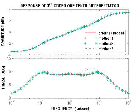
Fig.1. Frequency response of original and reduced 3rd order models of one-tenth differentiator

The frequency response of one-fifth differentiator using Carlson method (4) is compared with the response of the reduced 3rd order model obtained using the three methods in Fig. 2. It can be seen that the response of the model obtained using the three methods matches exactly with the frequency response of the original model in the entire frequency range [10-2,  102] rad/sec for both magnitude and phase plots, except a small range [100, 101] rad/sec in the phase plot.

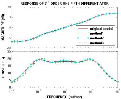
Fig.2. Frequency response of original and reduced 3rd order models of one-fifth differentiator.

The authors have also obtained reduced 2nd order models (Table 2) of the approximated integer order transfer functions of one-tenth and one-fifth differentiators. The simulations were performed and the results when compared with the original model did not show better performance.

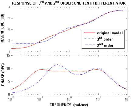
Fig.3. Frequency response of original and reduced 3rd and 2nd order models of one-tenth differentiator.

Fig. 3 shows the frequency response of one-tenth differentiator obtained using Carlson method and the response of reduced 2nd and 3rd order models using method 1. It is observed that the reduced 3rd order model shows better performance than the reduced 2nd order model as the former matches exactly with the response of the original model both in terms of magnitude and phase.

Similar analysis has been performed for all the approximate models listed in Table 1 and results compiled. Observations show that

• (i)    The performance of the reduced 3^rd order models using the three methods is superior to that of the reduced 2^nd order models. In our opinion this is due to the fact that the reduction up to 2^nd order affects a pair of dominant pole and zero, so the necessary characteristics and properties of original model are not preserved.

• (ii)    The Matched DC gain based reduced order models yield better results as compare to the models based on the other two methods.

  Table 1. Reduced 3 ^rd order models of fractional differentiator s^a (0 < a < 1)

  s "	Balanced truncation method	Matched DC gain method	Pade approximation method
  s 0.1	1.494 s 3 + 16.1 s 2 + 16.97 s + 1.455	1.487 s 3 + 13.92 s 2 + 11.24 s + 0.8046	1.494 s 3 + 9.301 s 2 + 6.057 s + 0.4168
  	s 3 + 14.19 s 2 + 18.69 s + 2.153	s 3 + 12.54 s 2 + 12.71 s + 1.202	s 3 + 8.69 s 2 + 6.925 s + 0.6227
  s 0.2	2.25 s 3 + 21.96 s 2 + 21.74 s + 1.66	2.236 s 3 + 19.01 s 2 + 14.07 s + 0.8572	2.25 s 3 + 17.56 s 2 + 10.95 s + 0.6421
  	s 3 + 16.92 s 2 + 26.07 s + 3.622	s 3 + 15.3 s 2 + 17.95 s + 1.929	s 3 + 14.73 s 2 + 14.29 s + 1.445
  s 0.3	3.361 s 3 + 26.29 s 2 + 20.47 s + 1.226	3.355 s 3 + 25.22 s 2 + 17.82 s + 0.981	3.361 s 3 + 4.077 s 2 + 0.508 s + 0.01678
  	s 3 + 18.43 s 2 + 27.88 s + 4.043	s 3 + 18.02 s 2 + 25.07 s + 3.297	s 3 + 5.291 s 2 + 1.111 s + 0.05639
  0.4 s .	5.063 s 3 + 29.71 s 2 + 13.85 s + 0.4578	5.086 s 3 + 33.61 s 2 + 22.01 s + 1.053	5.063 s 3 + 5.162 s 2 + 0.6023 s + 0.01879
  	s 3 + 20.28 s 2 + 25.2 s + 2.626	s 3 + 21.33 s 2 + 34.1 s + 5.333	s 3 + 7.311 s 2 + 1.687 s + 0.09513
  s 0.5	9 s 3 + 76.54 s 2 + 72.29 s + 4.117	8.961 s 3 + 64.51 s 2 + 38.29 s + 1.201	9 s 3 + 25.38 s 2 + 8.203 s + 0.2308
  	s 3 + 35.17 s 2 + 98.2 s + 27.46	s 3 + 33.38 s 2 + 67.91 s + 10.81	s 3 + 21 s 2 + 18.44 s + 2.077
  0.6 s .	13.45 s 3 + 56.36 s 2 + 9.465 s + 0.003083	13.52 s 3 + 74.39 s 2 + 39.08 s + 1.105	13.45 s 3 + 8.818 s 2 + 0.8156 s + 0.01725
  	s 3 + 34.35 s 2 + 42.75 s + 1.335	s 3 + 36.26 s 2 + 76.02 s + 14.85	s 3 + 15.9 s 2 + 3.995 s + 0.2319
  s 0.7	20.25 s 3 + 340.3 s 2 + 1280 s + 218.5	20.11 s 3 + 1127 s 2 + 2884 s + 96.94	20.25 s 3 + 11.04 s 2 + 0.9144 s + 0.01837
  	s 3 + 50.63 s 2 + 632.3 s + 1172	s 3 + 88.28 s 2 + 2084 s + 1963	s 3 + 22.65 s 2 + 5.934 s + 0.372
  s 0.8	30.26 s 3 + 438 s 2 + 1657 s + 204.7	30.17 s 3 + 574.5 s 2 + 1374 s + 36.66	30.26 s 3 + 11.79 s 2 + 0.8993 s + 0.01748
  	s 3 + 51.72 s 2 + 681.2 s + 1590	s 3 + 55.73 s 2 + 858.7 s + 1109	s 3 + 31.09 s 2 + 7.513 s + 0.5289
  s 0.9	45.56 s 3 + 617.9 s 2 + 2590 s + 175.6	45.52 s 3 + 621.3 s 2 + 1974 s + 40.51	45.56 s 3 + 12.07 s 2 + 0.7939 s + 0.01439
  	s 3 + 54.55 s 2 + 802 s + 2558	s 3 + 54.46 s 2 + 797.7 s + 1846	s 3 + 44.84 s 2 + 9.301 s + 0.6556

  
  

  Table 2. Reduced 2^nd order models of one-tenth and one-fifth differentiator

  s "	Balanced truncation method	Matched DC gain method	Pade approximation method
  s 0.1	1.494 s 2 + 12.78 s + 3.759	1.421 s 2 + 5.261 s + 0.5224	1.494 s 2 + 2.43 s + 0.1811
  	s 2 + 11.86 s + 5.065	s 2 + 5.481 s + 0.7805	s 2 + 2.707 s + 0.2705
  0.2 s .	2.25 s 2 + 17.99 s + 5.589	2.112 s 2 + 8 s + 0.7218	2.25 s 2 + 2.851 s + 0.1773
  	s 2 + 15.05 s + 9.579	s 2 + 8.339 s + 1.624	s 2 + 3.558 s + 0.399

  
  

  Table 3. Reduced integer order models of F FOP1 (s)

  order	Balanced truncation method	Matched DC gain method	Pade approximation method
  3	F FOP 1_ red _ BT ( s ) = - 0.0425 s 2 + 0.9587 s + 1.236	F FOP 1_ RED _ MDG ( s ) = 0.0077633 s 3 - 0.06249 s 2 + 0.9878 s + 1.288	F FOP 1_ RED _ PADE ( s ) = - 1.489 s 2 + 2.86 s + 0.3713
  	s 3 + 1.085 s 2 + 1.607 s + 1.26	s 3 + 1.907 s 2 + 1.624 s + 1.241	s 3 + 0.1195 s 2 + 3.088 s + 0.3754

  
  

• IV.    Illustrative examples

In this section we have picked up a fractional order plant [29] for simulation purposes. Each fractional term is substituted by second iteration Carlson approximated models and closed loop frequency and time responses of the plant is obtained for two different types of controllers.

• A.    Example 1a: Fractional order plant (F1)

A fractional order plant [29] is considered

F^{F 1( 5} )   0.8 s ²² + 0.5 s ⁰⁹ + 1

Each single term s^α of (21) is replaced by its corresponding Matched DC gain based reduced 3^rd order model from Table 1, and the integer order approximation F FOP1 (s) is obtained as

'      s ⁶ + 69.76.4 s ⁵ + 1649 s ⁴ + 1.503 e 4 s ³

+ 4.267 e 4 s ² + 3.467 e 4 s + 3561 __________ s ⁸ + 112.6 s ⁷ + 2290 s ⁶ + 1.678 e 4 s ⁵ + 4.489 e 4 s ⁴

₄ + 5.71 e 4 s ³ + 6.256 e 4 s ² + 3.694 e 4 s + 3600

The order of this transfer function is 8. Being of high order, it is further reduced using the three methods discussed in this paper and the final reduced model has order 3. The reduced integer order models obtained are given in Table 3.

The step response of the higher order integer approximation ( F FOP1 (s) ) and its reduced 3^rd order models ( F FOP1_RED_BT (s) , F FOP1_RED_MDG (s) , F FOP1_RED PADE (s) ) are compared as shown in Fig 4. It can be seen that the reduced 3^rd order model obtained using Balanced truncation method and Matched DC gain method show very close match with the higher order integer approximation, however Pade approximation method show very poor results.

The integer approximation of (21) obtained using another technique is given in [29, 30]. The step response of this approximation (shown as dashed line, F XUE (s) in Fig 4) is compared with the results obtained in this paper. It can be seen that the integer order approximation proposed in this paper matches very closely with the step response of the real system F_F1(s) (shown as ideal plot in Fig 4). This shows that the models developed in this paper are more close to reality.

• B.    Example 1b: Fractional order PD controller

A fractional order PD controller [29-31] to control the plant is chosen as

F_{f1 ro}( s ) = 20.5 + 3.7343 s ^1.15           (23)

The closed loop fractional transfer function of the system is

F F 1 ( s ) F F 1_ PD ( s )

^{F 1_ S B1 s} " 1 + F f 1 ( s ) F f 1_ PD ( s )

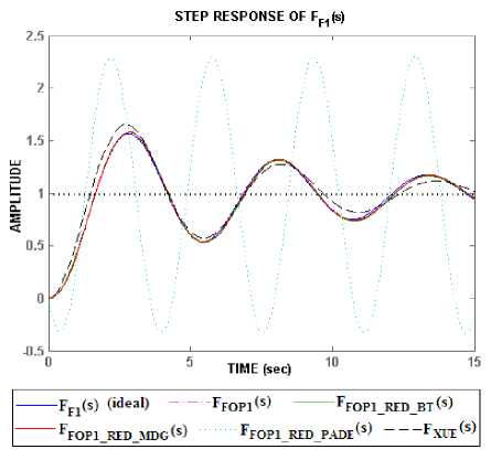
Fig.4. Comparison of step responses of higher and lower integer order models of F F1 (s) .

While analyzing the transfer function F_{F1_SYS1}(s) , we encountered three fractional term s^0.2 , s^0.9 and s^0.15 . For the term s^0.15 , α is 0.15. This results in 1/α being 1/0.15 = 100/15 , which is not an integer. Therefore, Carlson method of approximation cannot be used directly. As such, s^0.15 is decomposed as

0.15    0.1     0.05    10     20

sssss

.

The reduced integer approximation of s ^0.05 (obtained by using Carlson method and then reducing the order by Matched DC Gain reduction technique) used in the paper is

₀.₀₅ _ 1.218 s ³ + 11.98 s ² + 10.08 s + 0.7762

^s =    s ³ + 11.3 8 s ² + 10.72 s + 0.9482       ⁽  )

The fractional terms s0.2, s0.9 and s0.1 are substituted by its Matched DC gain reduced order model from Table 1, and the integer order approximation (FSYS1(s), not mentioned in this paper) of (21) is obtained. The order of this approximation comes out to be 20. Therefore it is further reduced using Balanced Truncation and Matched DC gain methods and the lower order models are given in Table 4.

The frequency and step responses of the higher order model ( F SYS1 (s) ), reduced order models ( F SYS1_RED_BT (s) , F SYS1_RED_MDG (s)) and the actual response ( F F1_SYS1 (s) (ideal)) are shown in Figs. 5a & b respectively. It can be seen that the performance of the lower order models are just the same as the higher order model. On comparison of the higher order model with the actual response there is no difference seen in the frequency response but some deviations are observed in the step response.

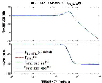
Fig.5a. Bode plots for comparison of the closed loop fractional order system model with fractional order PD controller

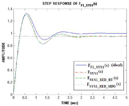
Fig.5b. Step responses for comparison of the closed loop fractional order system model with fractional order PD controller.

A fractional order PID controller [15, 30] to control the plant is

F, (нАs ) = 233.4234 + — 397- + 18.5724 s ¹¹⁵   (26)

The closed loop transfer function becomes

F

F 1_ SYS 2

( s ) =

F F 1 ( s ) F F 1_ PID ( s )

^{1 + F} F 1 ⁽ s ) ^F F 1_ PID ⁽ s )

To obtain the integer order approximation of the expression (27), the fractional terms s^0.2 , s^0.9 and s^0.1 are replaced by its approximate Matched DC gain method based reduced order model available in Table 1 and the term s^0.05 is substituted from (25). The integer order transfer function ( F SYS2 (s) ) obtained has order of 26 (not mentioned in the paper). The higher order model is now reduced to models of order 3 using Balanced truncation and Matched DC gain methods which are mentioned in Table 5, and their frequency and step responses are shown in Figs. 6a & b.

In [15], Xue et al. have simulated the same problem using different approximation and reduction technique. We have compared the response of [15] with the responses of the models proposed in the paper and also with the ideal response of the closed loop fractional order system F F1_SYS2 (s) .

The comparison is performed in two steps

• (i)    The lower order model of [15] (shown as “lower order model of ** [15]” in Figs. 6a & b) is compared with the lower order models of Table 5.

• (ii)    The higher order integer approximation of [15] (shown as “ ** [15]” in Figs. 6a & b) is reduced using Balanced truncation method (shown as “ F XUE_ _{RED_BT}(s) ” in Figs. 6a & b) and Matched DC gain method (shown as “ F XUE_RED_MDG (s) ” in Figs. 6a & b) and again these results are compared with the lower order model of [15].

• (iii)    From the observations shown in Figs. 6a & b it is evident that all the lower order models developed in this paper show very good results in terms of their closeness to the higher order model as well as to the ideal model (shown as “ F_{F1_SYS2}(s) (ideal) ” in Figs. 6a & b). Whereas, a noticeable difference is observed in the frequency and step responses of the lower order model of [15] in both the Figs. 6a & b.

  C. Example 1c: Fractional order PID controller

  
  

  Table 4. Reduced integer order models of F F1_SYS1 using the two methods.

  Order of the model	Balanced truncation method	Matched DC gain method
  3	3.825 s 2 + 29.27 s + 73.73 SYS 1_ RED _ BT ( s )   s 3 + 7.029 s 2 + 31.25 s + 77.7	0.004067 s 3 + 3.744 s 2 + 25.6 s + 51.02 FSYS 1 RED MDG ( s )         3 , r cm 2 ,     er -co c-> _   _             s + 5.849 s + 27.56 s + 53.53

  
  

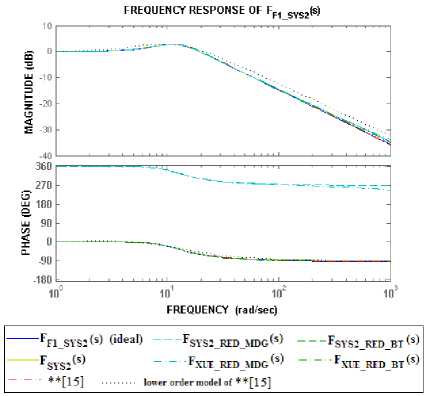
Fig.6a. Bode plots for comparison of the closed loop fractional system model with fractional order PID controller.

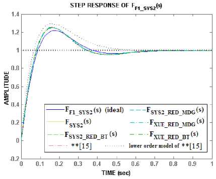
Table 5. Reduced integer order models of F F1_SYS2 using the two methods.

Order of the model	Balanced truncation method	Matched DC gain method
3	18.81 5 2 + 268 5 + 1337 ' 2_ RED _ BT ( 5 )   5 з + 23.28 5 2 + 270.9 5 + 1342	- 0.0009 5 3 + 18.87 5 2 + 279 5 + 1467 srs 2_ RED _ MDG ( 5 )       5 3 + 23.99 5 2 + 281.5 5 + 1473

Fig.6b. Step responses for comparison of the closed loop fractional system model with fractional order PID controller.

From these results, it can be inferred that – the Carlson method of approximation along with the reduction techniques viz. Balanced Truncation and Matched DC gain methods, yield responses which closely match the ideal response. Also, the reduction techniques used in this paper are better than the technique used in [15].

• V. Conclusion

In this paper we have developed reduced 3rd order integer-order models of Carlson method based fractional differentiators. For this, three model order reduction techniques are used viz. Balanced truncation method, Matched DC gain method and Pade approximation method. The performance of these models is verified by plotting their frequency responses. Through examples it is demonstrated that the technique used for order reduction is simple and effective. The simulation results show that the frequency response and step responses of the reduced order model matches very closely with the original models. Since even 3rd order is a very good approximation of a fractional order system, these models can be directly used for hardware realization. Further, the approximate models presented in the paper can also be used for designing fractional PID controllers, such as for speed control of PMSM and 3ΦIM which enhance the system performance.