Improved Image Retrieval with Color and Angle Representation

Published Online May 2014 in MECS

The development of information technology, and the increasing number of Internet users in addition to the spreading of social networks and video/image hosting websites, have a great influence on the tremendous growing of the digital media and image collections, a huge number of photos and videos are taken every day using digital cameras and mobiles to be uploaded later on the Internet.

These huge collections of multimedia are almost useless if we do not have the sufficient technique to retrieve specific data from this database depending on our information need, the strength of retrieving depends on the power of measuring the distance or similarity between two objects (images in our case).

The main two approaches used for image retrieval are the content-based and the text-based approaches shown in the following subsections.

• A.    Text-Based Image Retrieval (TBIR)

TBIR is the common and traditional approach; it is used in many search engines like Baidu, and Google. In this approach, images are annotated using keywords such as captioning, metadata, or descriptions added to the image database either manually by annotators or automatically by detecting tags and keywords around the image in the web page or the document; the first way is time consuming and needs great staff to annotate each image, while the second way is not guaranteed because it depends on any tag or word within the web page or the document, and so the similarity measurement will not be accurate, and it is highly expected to be irrelevant to the query. For example searching for the name of specific country will retrieve the flag, the map and may be the president as three similar or identical images for our information need.

The TBIR system works on reading documents and web pages to find images, then tags, annotations and keywords are extracted from the processed document to build a bag-of-words for this image, this process can be done in the offline mode, and the result will be a database with two main columns: the image ID and the bag of words describing the image.

However, TBIR is very powerful when we don't know the nature of the image, for example, if we do not know how the apple looks like, we can just write "apple" on the search engine to show a variety of images for different apples, but here, we have no difference between apple the fruit and apple the company.

• B.    Content-Based Image Retrieval

  The other approach is Content Based Image Retrieval (CBIR), which has been found in 1981 by Moravec [1], and some references consider the beginning of this field in 1992 by Kato [2]. The query in the CBIR is an image which used to retrieve images based on specific features like color, texture and shape, the term has been widely propagated to solve the problem of Text-Based Image Retrieval by retrieving images depending on image features instead of surrounding text or annotations, and because of its nature and power many researchers found that CBIR much sufficient for many applications more than the text based approaches [3-5], and because of its power many available search engines like Google, Yahoo and AltaVista added CBIR systems to their engines.

The main process in the CBIR depends on reading the images’ database or the collection, each image is converted from its original form into a signature that describes specific features in the image, this process is applied in the background of the server, or offline, and it does not affect the speed of the retrieving function, in the end of this process we will generate a signature for every image, this signature describes the image, and it has to be quite enough representative to be used in measuring similarity between two images.

The second part of the CBIR process is applied online, in this stage the client uploads his image to the CBIR system, this image is converted to a signature (in the same manner of the first stage), then this signature has to be compared to each one in our signatures’ database, then images are ranked and retrieved according to their similarity ratios.

The key challenge in CBIR is to represent the image as a value or series of values (the signature) that describe the image using its features, and then to measure the similarity between two images according to the generated signatures, the similarity measurement and enhancement depends on the type of features extracted from the image, in addition to the technique used to measure the similarity. So, the core work of CBIR research is to find the right way to extract specific and important features to represent the image as an object or signature composed of specific number of values, and then to use an adapted algorithm to measure the distance or similarity between two objects.

To measure the similarity many references used the color features, In [6, 7], similarity measurement in these references depends on the difference between the histogram of each image. Other researches divided the image into many regions according to the color of each region, then the color features or histogram is extracted from each region.

In the CBIR algorithm many factors must be taken seriously in our similarity measurement, these factors like the size of the new representation for the image, and the ability for compression, the time used to convert the image from its original form to the measurable data (the conversion of the whole database will be applied in the background as an offline process, but the conversion of the query image will be done online in the foreground), the ability to cluster these new representations (to increase the search speed), the ability to find the similarity between rotated or resized images, all these factors must be highly considered to build a powerful approach for image retrieval system.

• C.    Paper Organization

In the second section we are going to discuss the most important applications that depend on the content based image retrieval, then, in the third section we are going to show more about the history of the CBIR researches.

In the third and the fourth section we will describe our approach and our simulation results, with comparisons with many other techniques. In the sixth section we conclude the main ideas and results in our research.

• II.    Applications

In our rapidly-developing world, image retrieval is involved in many important applications like image searching and image indexing, used in search engines for retrieving similar images either from the internet or from local databases in a library or a hotel, or for police and intelligence uses.

Also image retrieval is used in medical diagnosis applications that depend on finding similar images (or parts within the image) to discover certain diseases and vulnerabilities. Photograph archives' applications also depend on retrieving similar images to be able to organize your archives and albums. Duplicate-image detection applications are also very important, these applications are used to discover if an intellectual property is abused, or used by someone else without citation.

Other applications like Architectural and engineering design, geographical information and remote sensing systems, object or scene recognition, solving for 3D structure from multiple images, motion tracking and crime prevention, all these applications depend on the ability of finding similar images within a collection.

The importance of the abovementioned applications and the huge collections of images has added more demand to develop a new branch of information retrieval called the “image retrieval” to enhance finding similarity among images using some features within the image.

• III.    Related Work

  The development of image retrieval using a set of features, or a group of points of interest, began in 1981, when Moravec [1] used a corner detector on stereo matching, this detector then was improved in [8] by Harris and Stephens to make it more sensitive to edges and points of interest in the image. In 1995, Zhang et al. [9] used the correlation window around the four corners of the image to select matches over larger collections, and then the fundamental-matrix for describing the geometric constraints has been proposed for removing outliers in the same research too.

Schmid and Mohr [10] started for the first time to use invariant local features matching for recognizing images. A feature was checked against a large database, their work was a development for [8], they used a rotationally invariant descriptor of the local region instead of the correlation window. In their research, they could make image comparisons invariant to orientation change between two images, they also proved that multiple feature matches could make better recognition under distortion and clutter.

Harris corners were very sensitive for change in scale. Lowe, in [11], enhanced the Harris corners approach to be scale invariant. Lowe used a new local descriptor also to make the approach less sensitive to local image distortions, such as 3D viewpoint change.

• A.    Color Features

In recent works, the color features started to be the dominant for researches in CBIR. Because CBIR systems are more interested in human visual system perception, the color layout descriptor and scalable color descriptor were used in the Moving Picture Experts Group MPEG-7 standard, but the main problem for color histogram and other color features is the disability to characterize image spatial characteristics, or color distribution, so many researches started to use other features like texture and shape in combination with color, because texture describes smoothness, coarseness and regularity of the image, which can be a good descriptor.

Combining many features and factors with the color feature explains two points, the first is the importance of the color feature for the human eye, and the second point is the weakness of color histograms when there is no spatial-dependent features are collected.

• B.    Texture Features

Because texture features are more descriptive for the real world images, many researches made more focus on texture, like Markov Random Field (MRF) model [12], Gabor filtering[13], and Local Binary Pattern (LBP) [14].

But the main problem with texture features is its weakness against any modifications applied on the image, like resizing, distortion or any type of noise. Texture based features, also, are not enough to measure the similarity between two images, because the smoothness or coarseness for two images does not mean that they are similar.

Another problem in the approaches that depend on the texture features is its complexity and its time-consuming process.

• C.    Objects Extraction

The Gabor filters [13] has been used in [15] to segment images into distinct regions, then features are extracted from each region separately instead of the whole image, then the Self-Organizing Map (SOM) clustering algorithm is used to group similar regions in the same class, in the same manner the query image is clustered and each region is compared with each centroid to find the region’s class, the class of each region is used later to find the similarity with other images composed of similar regions.

The problem in this approach is its log increasing function when the number of objects in the image increases, another problem is the similarity measurement approach that can be used to measure the similarity between two images, each with different number of objects.

• D.    Similarity using Descriptors Statistics

The MPEG-7 standard adopted three texture descriptors: homogeneous texture descriptor, texture browsing descriptor and the edge histogram descriptor [16].

In the texture features a new term, texton, was introduced in [17] that depends on the texture features. In [18], the authors proved that the human visual system is sensitive to global topological properties.

In [19], the Micro Structure Descriptors (MSD) was introduced. They depend on the underlying colors with similar edge orientation. The MSD extracts features and integrates colors, texture and shape information to represent an image for the retrieval process, the extraction process depends on structure elements shown in Fig. 1.

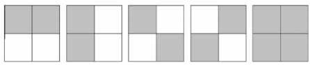
Fig. 1. Structure elements used to detect orientations in the image

In [19], statistics are gathered for the existence of every structure element in the image, these statistics are used later to build the signature and to measure the similarity between two images.

Two years later after [19], another approach was developed [20]. The new approach replaced the MSDs and used structuring elements histograms; the second approach showed good results compared to the first one with MSD.

The structure element descriptor in [20] is used to find the structuring elements histogram which represents the image's texture. The results in [20] are very promising and it deserves more work and development, but the main problem was its disability to discover similarities if translation, rotation or scale is applied to the image.

In addition to its disability to find similarity if the image was subject to any modification or noise, this approach is time consuming, because the system proposed in [19] depends on applying each structure element for each quantized color on each pixel in the image, so if we have 5 structuring elements, and 20 quantized color and a 200×200 pixels image, then we need to make a 5×20×200×200 operation before finding the structure elements histogram.

• E.    Recent Researches and Conclusive Remarks

Most of the new researches pay more attention to approaches that include the color features to adapt to the human visual system, the color histogram is an old approach but it still powerful, and some additions and enhancements (or adaptations) on the color histogram approaches can result in building a powerful CBIR system.

In [21] the researchers used the spatial relationship fuzzy color histogram (FCH), by considering the color similarity of each pixel’s color associated to all the histogram bins through fuzzy-set membership function. Instead of the conventional color histogram (CCH), which assigns each pixel into one of the bins only, FCH spreads each pixel’s total membership value to all the histogram bins.

Another approach in [22] used the color coherence vector (CCV), which partitions pixels based upon their spatial coherence. A coherent pixel is part of some sizable contiguous region, while an incoherent pixel is not. So two images with similar color histograms, will have different CCVs, if they were actually different.

In this research we will focus on fixing the weakness axis in the approaches that depend on the color histogram.

So, a novel approach will be used in this research, the main idea is to use a color/angle histogram to represent the image; this histogram is expected to be very descriptive for the image and to be scale invariant and rotation tolerant.

The approach will use a reference point in the center of the image for measuring the angle between vector A and Vector B, where vector A connects the center of the image with the point on the rightmost center of the image, and vector B connects the center point with our pixel.

• IV.    Proposed Approach

• A.    System Description

Our approach addresses two main problems in the CBIR system workflow, the first problem is the color quantization and the second is the representation of an image into a signature or series of representative values.

Color quantization is a very important process for any CBIR system, and it is the first process to be applied to the image before extracting the required color features, in [23] the authors focused on the quantization problem and its impact on the CBIR performance. The two common approaches used for quantization are the uniform and non-uniform color quantization. In our approach we will quantize the colors of the image into 37 colors using the non-uniform color quantization techniques.

To convert an image to a color and angle histogram (CAH) or the signature, in our proposed approach, we divide an image into a number of angles, then statistics for the number of each quantized color in each angle are gathered to make the required signature. The signature generation is not enough but also we have to choose the right technique to measure the similarity between two signatures, a measurement technique is also proposed in this paper.

To enhance the operation of the proposed CBIR system a rotation resistant technique has been added, this technique will make our CBIR system able to detect similarity between images even if they were rotated.

To increase the retrieval speed for the CBIR system a clustering algorithm will be used, after this step a query image will be compared with the centroids of the clusters instead of measuring similarity with each image in the database.

In the second part of the process we have to find the CAH for the query image and to use our proposed similarity approach to find the distance between each CAH in the database and the CAH of the query image, then images are retrieved and ranked.

• B.    Non-Uniform Color Quantization

The number of colors within any image depends on the image type, color system and the depth of the color per pixel, for example if the RGB system used, with 8-bit depth for each color, then, our image includes 224 colors or 16 million colors. The first problem is that processing the image with all the possible colors needs high computations, which makes more complications for image retrieval applications, this problem can be solved by decreasing the number of colors in the image to a small number that does not make high computations in the image processing stage. The second problem with this huge number of possible colors in the image is the difference between two similar colors, for example two colors with two different saturations will look different for the computer vision, but for the human vision they might look as one color. The solution for the second problem is to consider looking-similar colors as one color.

The solution for the two abovementioned problems is to use quantization, which is the process of defining blocks of similar or close colors as one quantized color, this process will decrease the number of colors from millions to dozens, and many colors with different grades will be treated as one color, this process will decrease the computation time, which is our first goal, and it will increase the power of our CBIR system.

To quantize a specific color system we have to define our criteria, for example in the RGB system we can define all the colors with ( R<50, G<50 and B<50 ) as black, we can also define specific value for the white color, for example if (R>200, G>200 and B> 200) the color is considered white, but the RGB color is very good in the computer vision, but it differs very much from the human vision system which depends on perceiving the color and its saturation, the closest color system for this is the HSV system, so we will use the HSV color system for our quantization process.

From [15] we can use equations (1), (2) and (3) to convert the RGB color system to an HSV system:

Н = arctan  ^(G ^(1)

(R - G)+ (R - В )

• v = RF)(2)

„ _ , min{R,G,B)

• 5 = 1 —    у

• The human eye color-perception system is very close to the HSV color space distribution, so it is expected to be very powerful in the content based image retrieval applications, and it is used in almost all the CBIR systems to retrieve similar images, The HSV color divides the color into three values, Hue H (Hue is represented as a disk from 0 to 360 degrees), Saturation S (0 to 1) and Value V (0 to 1), these values are illustrated in Fig. 2.

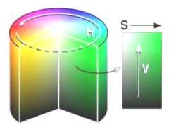
Fig. 2. HSV color space

The Hue elaborates the distribution of the colors, similar colors for the human vision are located as adjacent colors on the Hue disk, for example the similarity between the Blue and Cyan colors for the human vision system is very high, and the two colors are adjacent in the Hue colors distribution.

Colors with low saturations are light and look like white for the human eye, and colors with low values look like black for the human vision system.

Different quantization systems used in CBIR applications, most of these applications depend on the uniform quantization for the HSV space, in these approaches the Hue is quantized into a number of periods, each period is substituted by a new number, for example if we assume the Hue is distributed across a disk like Fig. 2, Then the disk is divided into uniform slices each is 60 degrees for example, these approaches that depend on the uniform quantization suffers some problems. In our proposed approach we depended on the non-uniform color quantization, which does not depend on similar angles.

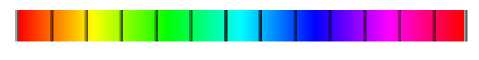
(a) The Hue Colors Distribution

(b) Uniform Color Quantization

(c) Non-uniform Color Quantization

Fig. 3. Hue color quantization

Fig. 3 (a) shows how the distribution of the colors across the HSV disk, the colors appear to be non-uniform, that makes the traditional quantization algorithms that divide the H space into similar pieces inaccurate.

Fig. 3 (b) and (c) illustrates the quantization blocks in the uniform and non-uniform quantization.

Fig. 3 shows that the main colors of red, green and blue occupies more H-space than the other colors like Yellow, Cyan and Pink do, so we can use i.e. 80 degrees for the blue color and 30 degrees for the pink color to solve this problem, which is called the non-uniform color quantization.

So, in this step it is not fair to divide the H plane into same-size pieces or blocks. Some ideas excerpted from [24] will be used in this paper for quantizing colors, the first idea is to divide the Hue plane into non-equal blocks according to the spread of each color, the second idea is to depend on the Saturation and the Value for the first step in the quantization process, in the first step the quantized color is classified as white, black or gray. The results showed that the ideas in [24] can make very good results but with some modifications on the Hue plane segmentation and more work in detecting the intervals of the first step quantization.

Another good quantization technique has been used in [20], this approach does not divide the Hue, Saturation and Value into similar blocks, but it depends on the distribution of the color to quantize it, and it depends on the darkness to consider whether the color is black or white.

Another idea is used in the non-uniform color quantization to quantize the Saturation and Value plane, to understand this approach we have to understand Fig. 4 that shows the SV plane for three colors, Red, Green and Blue, Then Fig. 5 will make more illustration for the quantization process.

From Fig. 4 we have to note that low saturated colors look like white, and low valued colors look like black, and other notions will be discussed on Fig. 5

Saturation Increasing »

Saturation Increasing »

Saturation Increasing »

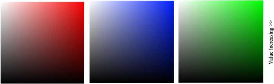
Fig. 4. Saturation and Value planes

Fig. 5 describes the SV space for saturation and value (the figure used the Red color, and it is applicable for the other colors), it is obvious from the figure that the low values are perceived by the human eye as black (Area 1), because of its darkness, the main idea here is to quantize all colors with V<0.2 as one color, so the darkness of the color will be used to detect black colors with ignoring the main color Hue and Saturation in this step, this makes our work very close to the human vision system, because it is another problem in the uniform color quantization approaches that they depend on giving more importance to the Hue color [25], while the non-uniform color quantization depends on the value of the Hue, Saturation and Value to decide which color has to take the power in the quantization process.

Another observation in the SV space is the gray area when S<0.2 ( Area 2), in addition to the bright area which can be quantized as one color(white), the intended area is labeled 3.

In Area 2 the saturation S<0.2 and the Value V<0.8 and V>0.2 , all the colors with these characteristics ( the hue is ignored ) will be considered as gray. In Area 3 where S<0.2 and V>0.8 the color is quantized as white color, if the conditions of Area 1, 2 and 3 are not matched, then the Hue will be used as the main value for our quantization. The remaining region is the real color region, which can be quantized as a combination of the three attributes H,S, and V.

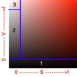
Fig. 5. SV plane quantization

The quantization steps can be described as the following steps, where C is the final value of the quantized color:

1.    с=0,for v∈[0,0.2]

This is area 1 in the bottom of Fig. 5, from the color of this area it is obvious that it has to be quantized into one black color with C=0.

• 2.    for sϵ [0, 0.2] and v ϵ [0.2, 0.8), C is quantized to a gray color:

• 3.    when s ϵ[0.2,1] and v ϵ(0.2, 1] it is a real color area, in this area the colors are segmented as shown in Fig. 3 (c). In this step the first thing we have to do is to quantize each plane in the HSV planes into a specific number of values. Saturation and Value will be quantized into 2 values (0, 1) for each, the Hue will be quantized into 7 values (0, 1, 2, 3, 4, 5, 6), as shown in the following steps:

C = floor((v – 0.2)×10) + 1

This step quantizes area 2 in Fig. 5, this area is gray gradient, it changes from the dark gray to the light gray as v increases. In the above equation the max value of v is 0.8, which will result in ((0.8 -0.2))×10) + 1 = 7, and the minimum value of v is 0.2, which will result in ((0.2 -0.2)×10) + 1 = 1, Now we understand that this step makes a result in the period [1, 7], where 1 means dark gray, 7 means light gray and other values like 2, 3, 4, 5, 6 are just gray level gradients.

In this step we used the floor to convert numbers into digits only, we also added 1 to the equation to avoid the result C=0 which means the black quantized color.

• a.    S = 0 if s ϵ(0.2,0.65] and S =1 for s ϵ (0.65,1]

• b.    V=0 if v ϵ(0.2, 0.7] and V =1 for v ϵ(0.7,1]

The following formulas elaborate the quantization of the Hue spectrum (as seen in Fig. 3 (c)):

• 2,    Hϵ[0, 22] U Hϵ (330, 360], (Red Color).

• 1,    Hϵ(22, 45], which is Orange.

• 0,    Hϵ(45, 70], which is Yellow.

• 5,    Hϵ(70, 155], which is Green.

• 4,    Hϵ (155, 186] ,which is Cyan.

• 6,    Hϵ (186, 260] , which is Blue.

• 3,    Hϵ (260, 330], which is the Purple color.

• 4.    When s ϵ[0, 0.2] and v ϵ(0.8, 1] , which is area

Now the Hue value is quantized into 7 values from 0 to 6, these values are arranged to make close colors next to each other, i.e. the yellow color is closer to the orange for the human eye, so they are close to each other in the quantization.

The final measurement of the color C is:

C = 4H+2S+V+8                        (4)

Where H stands for quantized Hue values in the range [0, 6], S for saturation and V for Value. The quantization of the main color area will result in 28 colors (from 8 to 35), we added 8 to our equation to avoid the results in step 1 and 2 where C=0 (black color) and C= (1, 2, 3, 4, 5, 6, 7) for the gray level gradients.

In (4) the first quantized color will be 8 (when H, S and V are zeros) and the last one will be 35 (H=6, S=1 and V=1).

number 3 in Fig. 5, this part is quantized into a white color and C=36. And then we have a total of 37 colors, from 0 to 36.

• A.    Representing image as Color and Angle Histogram CAH

The main idea in this step is to select a reference point in the center of the image, then according to this point the image is divided into 8 regions (We used 8 regions in our CBIR system, but other divisions can be used), these regions will make our CBIR system able to detect rotated images if the rotation was in the increments of 45°, Fig. 6 illustrates the meaning of the angles in this context.

Fig. 6. Image is divided into 8 regions

Then the image representation process has to count the number of each quantized color in each angle, to convert the image into a color and angle histogram (the proposed CAH signature).

The following example divides the image into 4 angles, and 3 quantized colors to describe the process of the proposed technique. The angles are quantized in this example as follows:

• 1.    0 to 90 is quantized as 0

• 2.    90 to 180 is quantized to 1

• 3.    180 to 270 is quantized to 2

• 4.    270 to 360 is quantized to 3

Now if we have two vectors U and V , with U is a horizontal vector extends from the reference point in the origin and the farthest point to the right, and V is the vector extends from the reference point in the origin and our point of test P (x 1 , y 1 ) , then (5) will be used to find the angle between the two vectors:

Z1 —   n -1 ^xi~° . —

= tan       = tan                         (5)

У1-0           yi                          v ’

Then Ɵ is quantized to the four abovementioned values (0, 1, 2 and 3) according to its value.

For this elaboration assume that we used the center point as the main point, and assume that the image was quantized for 3 arbitrary colors ( 0,1,2 ), and let the angel be divided into 4 regions as shown in Fig. 7 (b) , then let Fig. 7 (a) is the quantized and processed image.

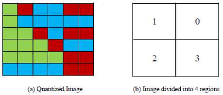
Fig. 7. Image quantized into three colors Red = 0, Green = 1, Blue = 2

The color/angle histogram (CAH) will be represented as shown in Fig. 8, in the first row number 4 (in the first cell ) means that there are 4 pixels colored red and fall in the angle between 0 and 90 degree, the number 3 in the first row (in the last cell) means the number of blue pixels that falls in the angle from 270 to 360. The first row (the grayed row) will represent the final CAH signature in the end.

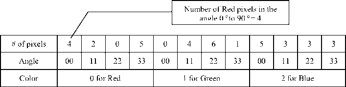
Fig. 8. The final CAH for the image (the gray row)

Histogram will be represented in x values, where x is the result of multiplying the number of quantized colors and the number of the quantized angles. In our example we have three quantized colors and 4 angles, so we have 3×4 values or 12.

In the real application, the number of quantized colors will be 37 colors and the number of angles will be 8 angles(total number of CAH values =37×8 = 296 value).

In the previous example the image is represented as the vector (4, 2, 0, 5, 0, 4, 6,1,5,3,3,3), this vector will be used later for measuring the similarities among images.

However, to make this Color and Angle Histogram (CAH) invariant to scale changes we have to make all the numbers in this CAH in the period [0, 1], this can be achieved by dividing all the numbers by the maximum number in our CAH, which is 6 in our example, and other techniques will be used in section 4.4 to make a rotation resistant CAH.

• B.    Rotation Resistant CAH

One of the important goals for any CBIR system is to be able to detect similarity between an image and its rotated copy, and the power of this rotation invariant system depends on the rotated angles that can be detected, for example some CBIR systems can detect flipped images (horizontally or vertically) only, other approaches can detect images if rotated 90° or its multiples (90°,

180°, 270° or 360°). This Rotation invariant CBIR system needs additional techniques or modifications for the image or the signature.

The histogram or CAH must be adapted to be tolerant for specific incremental rotations and to be scale invariant too, in the end of the previous section we illustrated how to make this CAH scale invariant, now we are focusing on the rotation invariance problem, to fix this problem we will find the highest value in the CAH, which is 6 in our example, this value has to be rotated to be the first in the group ( 0 ,4 ,6 ,1 ) ( in the previous example we divided the image into 4 angles) , so it has to be rotated two steps to left, the new block will be (6, 1, 0, 4), and all the other colors has to be rotated two steps too, so the histogram will look like the array (0, 5, 4, 2, 6 , 1, 0, 4, 3, 3, 5, 3), this rotation for each image in the collection will make the similarity measurement resistant for rotations in any angle of the sampled angle (which is 90° in our example and 45° in our approach), in our approach rotating the image to 45°, 90°, 180° or 270° will result in the same vector (with some differences because of the distribution of the pixels), this will make the similarity high between the original image and its rotated copy.

The rotation of the CAH is not applied on the whole vector (the CAH), it is applied on each block (each block represents a color), so we have to make 37 rotations one for each block.

• C.    Similarity Measurement

Each Image is represented as an array of values (the CAH), each value lies in the range [0, 1], The Euclidian Distance ( and the simplified form of it without the square root) has showed insufficient results in many tests, the main reason of weakness in this method is its equality in measuring differences, for example the distance between the following couples ( (0, 0.2), (0.4, 0.6) and (0.8, 1)) is 0.2 for each couple, but this is not perfect, because the value of the numbers has different impact on the similarity measurement (higher numbers have more impact than small numbers that might be just noisy colors). (6) is used to measure the Euclidian distance:

^| X ^- У |= √∑ "=i⁽ xt ^- У1 ^{) 5}                      (6)

The main argument in our approach with the Euclidian distance is that zero and low numbers do not deserve the same interest of high numbers in our calculations.

Another similarity measurement like the chi-square distance (7) from [26] added the sum of the two values to the denominator, this addition will increase the similarity when the two values are the higher, and vice versa the similarity will be lower when the two values are lower.

dissimilarity = ∑ь^.5 ( ⁽ ; ) ⁾ + Ft ( ₍ ■ ⁾ ₎ /               (7)

However the above distance measurement formula (7) needs more modifications to match our idea, and it also has to avoid the zero value of the denominator, when the two values are zeros.

In the modified technique used in this research, the similarity is adjusted to make non-uniform distances according to the effect of each value in the represented image. Note that in the following equations we depend on the concept of similarity and not the distance (like the Euclidian and the chi-square distances), so, two identical images have the similarity 1, and two totally different images have the similarity value of zero.

In our similarity measurement the result is a variable number in the period (-∞,∞), in the end of the calculations the results will be converted to be in the period [0, 1], with 0 is two different images and 1 means two identical images.

The similarity s _i measurement between two values a _i and b i in two vectors A and B is calculated as follows:

• a)    If a i or b i equals zero

s i = - |a i -b i |                                                      (8)

• b)    If a i and b i ≠ 0

s i = (1-|a i – b i |) × min(a i , b i );                        (9)

In (8) the difference between two values with one of them is zero is considered as a negative similarity, because in each value in the first image must has a response in the 2nd one, if there is no existence for this color in this angle it is considered negative response. Note that this condition can never exist in two identical images.

In (9) the similarity is multiplied by the lowest number to make low importance for small numbers like 0.1 and 0.2 when it has to be compared with 0.88 and 0.92 for example, and to give less importance for comparisons between 0.9 and 0.07 for example ( considering the small values are expected to be noise).

where the total similarity S is shown in (10) , i is the location of the feature in the vector, and n is the number of values in the signature of the image or the CAH in our research.

• S= ∑ i=l^st (10)

After measuring the similarity between the query image and each image in the database, similarity then is converted to be in the range [0, 1] with 1 means identical images, and 0 means no similarity at all.

After retrieving a number n of images, the similarity between each retrieved image and the query image is saved in the vector R = (r 1 , r 2 , ……, r n ) , where r 1 is the similarity between the first retrieved image and the query image.

From the similarity measurement equations 8, 9 and 10 we know that the values in the vector R are not located in a specific period, and this problem has to be solved to be able to rank the images later.

The equations used to normalize the vector of results R to be in the period [0,1] are as follows:

• 1.    R – min(R) , Convert all the values in R to be in the period [0, ∞), no matter if the lowest value is positive or negative.

• 2.    R / max(R) , this will convert all the values in the results vector to be in the period [0,1], because the maximum value has been divided by itself to be 1, and all the other values will be ≤ 1.

The results of our calculations are similarities, and they can be converted to distances only by making the subtraction 1-R.

The above similarity measurement showed an enhanced results in retrieving images in the proposed system, in the simulation and results section, there is a comparison between our proposed similarity and the results of the Euclidian Distance similarity.

• V.    Simulation and Results

• A.    Experimental Environment

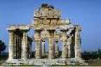
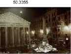
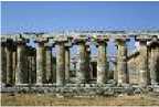
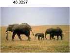
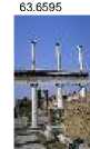
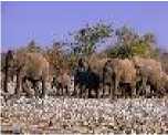
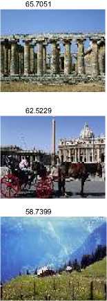
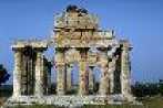
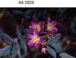
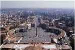
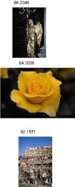
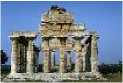
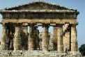
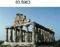
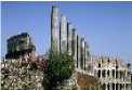
  The Corel 1000 images database which includes 1000 images has been used as the dataset to find the ratio of the image retrieval success for the ten types in the database ( Africa , Beaches, Building, Buses, Dinosaurs, Elephants, Flowers, Horses, Mountains and Foods), the database includes 100 images from each type, Fig. 9 shows a sample of the Corel 1000 images database.

In the first step Matlab code has been written to read the whole database and convert each image to the representing vector, or the CAH, which depends on the color and angle, the output is saved to a text file, then the query image has to be represented in the same way, and the resulting vector has to be compared with each vector in the text file, the Matlab code has been adapted to generate the CAH signatures using either the uniform or non-uniform color quantization techniques.

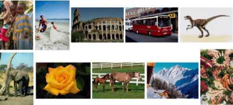
Fig. 9. Corel 1000 images database samples

To find the precision of our system for each type of images, 10 images are selected from each type randomly as query images, the search algorithm will start and retrieve the top 20 images with the highest similarity (for each image of the 10 images), then the precision value is measured (how many relevant image retrieved in the top 20 images), the average for the ten images is considered as the final precision value for the type of images.

The results showed very good enhancement in finding similarity among different types of images, for other types the enhancement was slight because of the interference among similar colors in some types of images.

In the following sections we will work on comparing the CBIR system using uniform and non-uniform color quantization techniques, we will also compare the results when using the Euclidian distance and our proposed similarity measurement technique.

To add noise and make some modifications on the images like rotation, translation and resizing, the well-known image processing application Adobe Photoshop was used.

The laptop used for building and running the codes is an i7 CPU with 2.4 GHz core 2 quad, and 4GB RAM.

• B.    Color Quantization and Similarity Measurement

In this part we tested our approach using 4 different combinations; in the first test we used the uniform color quantization and the Euclidian distance for similarity measurement. In the second test, we used the nonuniform color quantization, and the Euclidian distance for similarity measurement, in this test we witnessed a good enhancement on the results, which means that our proposed quantization technique is effective.

In the third test we used the uniform color quantization and our proposed similarity measurement approach, in this test better results are shown, which means that our proposed similarity measurement is making good enhancement for the CBIR system.

In the fourth test we used the two proposed techniques combined 1) the non-uniform color quantization, and 2) the similarity measurement approach, in this test we got our best results.

Table 1 illustrates the comparison between the four abovementioned tests.

Table 1. Precision Ratios Comparison

	UCQ precision using ED	NUCQ precision using ED	UCQ Precision	NUCQ precision
Africa	0.264	0.328	0.539	0.756
Beaches	0.357	0.419	0.482	0.532
Buildings	0.411	0.527	0.544	0.613
Buses	0.357	0.729	0.715	0.878
Dinosaurs	0.905	0.917	0.869	0.9934
Elephants	0.504	0.859	0.643	0.881
Flower	0.614	0.827	0.688	0.855
Horses	0.731	0.759	0.879	0.938
Mountains	0.251	0.314	0.482	0.527
Foods	0.352	0.529	0.548	0.649
Average	0.4746	0.6208	0.6389	0.76224

From the previous results in Table 1 we can conclude that the non-uniform color quantization adapted in this approach has made better retrieval results in our CBIR system, and we have to note that the used uniform color quantization is an adapted technique that works smarter than the traditional uniform quantization technique, but eventually, our technique could overcome this smart adapted quantization technique.

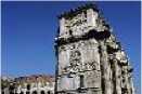
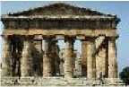
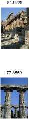
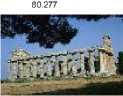
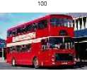
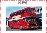
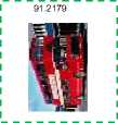
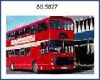
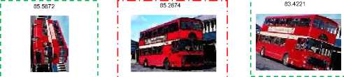
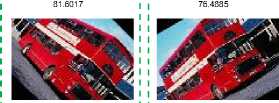
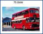
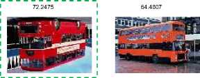
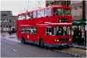
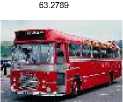
Fig 10, 11, 12 and 13 show some samples of the results made in the four tests, where the left upper image is the query image retrieved with similarity of 100%.

In Fig. 14 a query image of a bus is used, this image was subject to translation, resizing, rotation in addition to other noise effects, all the variations of the modified images were added to the Corel 1000 images database, then we used the query image (mentioned above) to retrieve the relevant images, in this test, all the modified images are retrieved which means that our approach was able to detect the query image even if it was a subject to many types of modifications.

In Fig 14 the red rectangle means query image with added noise, green rectangle - - means rotated image, blue rectangle – includes translated image, and orange (dotted) rectangle …. includes the zoom out of the original image.

In the previous comparisons we used the top 20 retrieved images to measure the precision ratios, in the next comparisons we will measure the precision ratio for different numbers of retrieved images, to make this comparison we will select 10 random images from each type of images in the Corel 1000 images database (the database includes 10 types of images, return to Fig. 9), so the total number of selected images will be 100,for each type of images we will find the relevant images in the top 5, 10, 20 and 30 images, then we will take the average for every 10 images from the same type to consider this average as the final precision ratio for each type.

Table 2 shows that we got high precision ratios when we make our measurements on the top 5 retrieved images, the precision ratios have decreased for larger numbers like 10, 20 and 30.

However, in our research we used the values in the third column (20 images), to compare our results with other researches, because the top 20 images retrieved were used in the other researches, and they are the most interesting retrieved images for the client (we suppose that).

Table 2. Comparison between different precision ratios for different number of retrieved images

	Top 5 relevant	Top 10 relevant	Top 20 relevant	Top 30 relevant
Africa	0.885714	0.814	0.756	0.417
Beaches	0.8	0.739	0.532	0.389
Buildings	0.76	0.693	0.613	0.429
Buses	0.92	0.892	0.8788	0.79
Dinosaurs	1	1	0.9934	0.908
Elephants	0.971429	0.843	0.4459	0.382
Flowers	0.914286	0.904	0.855	0.788
Horses	0.9824	0.972	0.938	0.81
Mountains	0.7388	0.7019	0.527	0.48
Foods	0.8926	0.7693	0.6495	0.52

Before the end of this section we can talk about the time used in different steps of this system (using an i7 2.4GHz CPU and 4GB machine):

• 1.    Time used to convert all the Corel-1000 images into CAH signatures text file was 15 minutes for 1000 images (less than 1second per image).

• 2.    Time used to compare a CAH signature with all the signatures was ≈ 0 seconds.

• 3.    Time used to upload an image, compute its CAH and measure similarity with all the signatures and retrieve the result of top 20 images is less than 1 second.

The query image and all the images can be resized to predefined size (smaller than the original), this preprocessing step can decrease the time used in finding the CAH, and it has an intangible effect on the retrieval efficiency.

Table 3 shows some comparisons between our proposed approach and other results from different researches, but we have to notice that the time consumption depends on the used machine specifications.

• C.    Comparison with other Approaches

Table 4 elaborates the comparison of the proposed technique with other techniques used in previous researches, the results showed significant optimization in many types of images.

Table 3. Average retrieval time for different approaches

Approach	Proposed Approach	ERBIR with SOM [15]	ERBIR without SOM [15]	Fractal Coding Signature [27]	MSD [19]
Retrieval time Average/second	0.9	0.23	0.78	1.766	Not available

Table 4. Comparisons with other CBIR systems precisions for the top 20 retrieved images

	Fuzzy Club	IRM	Geometric Histogram	Signature Based CBIR	Modified ERBIR	Proposed Technique
Africa	0.65	0.47	0.125	0.42	0.7025	0.756
Beaches	0.45	0.32	0.13	0.46	0.57	0.532
Building	0.55	0.31	0.19	0.25	0.4925	0.613
Buses	0.7	0.61	0.11	0.83	0.8675	0.8788
Dinosaurs	0.95	0.94	0.16	0.92	0.9925	0.9934
Elephants	0.3	0.26	0.19	0.95	0.5725	0.881
Flowers	0.3	0.62	0.15	0.96	0.835	0.855
Horses	0.85	0.61	0.11	0.89	0.9275	0.938
Mountains	0.35	0.23	0.22	0.32	0.4975	0.527
Foods	0.49	0.49	0.15	0.28	0.655	0.6495
Average	0.559	0.486	0.1535	0.628	0.71125	0.76237

Table 4 compares our results with other approaches like IRM [28], Fuzzy Club [29], Signature Based [30], Geometric Histogram [31] and ERBIR [15].

From Table 4 we can see that our proposed approach could overcome the other approaches in many cases.

In the end of this section we can conclude that representing an image as a color and angle histogram or signature is a very powerful approach in CBIR systems, and the comparisons proved that our approach using the proposed non-uniform color quantization technique and our proposed similarity measurement is a promising approach and can be used in many and different types of CBIR systems.

The results also showed that our approach is much better than using techniques like the color histogram in its traditional form, the results also showed that our approach is a scale invariant approach because the CAH is normalized, which makes the size of the image not a concern, and this solves the problem of using texture based or object based approaches. Another achieved goal is that our approach is able to tolerate specific rotations according to our angles' divisions, which make the system able to find the image if rotated with specific degrees or if flipped horizontally or vertically.

• VI.    Conclusion And Future Work

47.8993

In this research a new idea is proposed to represent a colored image as a signature describes the color and angle distribution for each color within the image. The first step in this approach depends on quantizing the image into a number of colors; this step eliminates the number of the colors in the image from millions to dozens, which makes the other steps simpler and faster. The quantization operation also makes the process more accurate, because it makes our system ignores fine gradients in the image; that will make the blue sky looks as one color instead of thousands of similar colors.

47.5179

45.0562

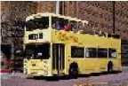
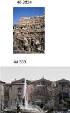
Fig. 10. Euclidian distance and uniform color quantization test

45.8576

44.1866

45.3515

44.1852

81.7089

79.6088

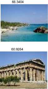
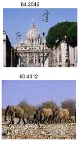
Fig. 11. Euclidian distance and non-uniform color quantization test 1

59.6847

67.9857

65.7449

63.7265

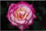
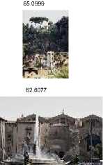
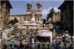
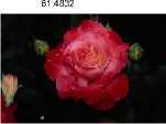
Fig. 12. Proposed similarities and Uniform color quantization

82.433

78.9813

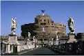
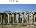
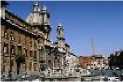
Fig. 13. Proposed similarity and non-uniform color quantization

The non-uniform color quantization technique used in this research is very close to the human eye vision system, which makes the CBIR system works closer to the human eye system.

Comparisons between the CBIR system using this quantization technique and other traditional techniques showed that this technique is more accurate and simulates the human eye in its mechanism, the numbers showed good and interesting results using this approach.

The second step in our CBIR system divides the image into a number of regions, then, for each region, the number of each quantized color has to be found to make a histogram for each division, then a complete color and histogram CAH representation for the whole image will be the concatenation for all the generated histograms for each angle.

This CAH will make the CBIR system depends on the color and the location of the pixels in the image, this will overcome traditional color histogram systems that depend on the whole image as a unit.

To measure the similarity between two signatures we used a new proposed similarity measurement technique, the proposed technique showed results much better than the traditional Euclidean distance.

The results and comparisons with other CBIR approaches showed that our proposed technique was efficiently able to detect similar images for different types, colors and sizes; the results showed that this technique could overcome many other CBIR techniques and can be used as a reliable and efficient technique for retrieving similar images depending on their contents.

The proposed technique is able to tolerate rotated or resized images, and rotated images in 45° increments are retrieved with high similarity values, identical images are retrieved with similarity of 100% which makes it more efficient in finding identical images. Also when some noise or modifications are applied on the image, the system is able to retrieve these images.

The comparisons and results show that our approach overcomes many other approaches like Fuzzy Club, IRM, Geometric Histogram Signature Based CBIR and Modified ERBIR, in almost all the tests.

In terms of time and space the technique was not consuming because the conversion of the images can be done in the background without impacting the client's time, and the representatives of the images are simple vectors that can be compressed with the traditional compression techniques.

The converted database can be clustered to get more efficient and time efficient retrieval for image retrieval systems with huge databases, after clustering the similarity measurements will be done between the query image representing vector and each centroid instead of measurements against all the images in the database.

64.3621

64.2606

59.6658

58.9108

57.4571

Fig. 14. Bus image with different modifications: rotation, translation, resize and additional noise