Improved Krill Herd Algorithm with Neighborhood Distance Concept for Optimization

Автор: Prasun Kumar Agrawal, Manjaree Pandit, Hari Mohan Dubey

Журнал: International Journal of Intelligent Systems and Applications(IJISA) @ijisa

Статья в выпуске: 11 vol.8, 2016 года.

Бесплатный доступ

Krill herd algorithm (KHA) is a novel nature inspired (NI) optimization technique that mimics the herding behavior of krill, which is a kind of fish found in nature. The mathematical model of KHA is based on three phenomena observed in the behavior of a herd of krills, which are, moment induced by other krill, foraging motion and random physical diffusion. These three key features of the algorithm provide a good balance between global and local search capability, which makes the algorithm very powerful. The objective is to minimize the distance of each krill from the food source and also from the point of highest density of the herd, which helps in convergence of population around the food source. Improvisation has been made by introducing neighborhood distance concept along with genetic reproduction mechanism in basic KH Algorithm. KHA with mutation and crossover is called as (KHAMC) and KHA with neighborhood distance concept is referred here as (KHAMCD). This paper compares the performance of the KHA with its two improved variants KHAMC and KHAMCD. The performance of the three algorithms is compared on eight benchmark functions and also on two real world economic load dispatch (ELD) problems of power system. Results are also compared with recently reported methods to establish robustness, validity and superiority of the KHA and its variant algorithms.

Еще

Krill Herd Algorithm (KHA), mutation and crossover, neighborhood distance concept, unimodal function, multimodal function, economic load dispatch

Короткий адрес: https://sciup.org/15010874

IDR: 15010874

Текст научной статьи Improved Krill Herd Algorithm with Neighborhood Distance Concept for Optimization

Published Online November 2016 in MECS

Optimization is basically a spontaneous process that plays an important role in real world application. Its objective is to compute a set of variables that either minimize or maximize the objectives function within given constraints. For solution of a given model or an objective function, there is a need of efficient optimization techniques which can either be conventional (deterministic) or have a stochastic, evolutionary approach. Conventional techniques include nonlinear programming, linear programming, quadratic programming, Newton’s method etc. Deterministic approaches generally require an initial guess which has a vital impact on the final solution. Considering practical utility of optimization there is need of robust and efficient algorithms which are free from this limitation.

Generally the practical problems are much complex and also have many constraints which cannot be solved by conventional approaches. On the other hand, nature inspired methods which are basically population based stochastic search techniques often provides quick and reasonable solution; though a careful tuning of parameters is required to prevent solution from getting trapped in local minima. In the recent years various population based evolutionary techniques have been developed for solution of problems related to real world application.

Among evolutionary algorithms genetic algorithm (GA) is probably the most popular algorithm based on Darwinian evolution concept proposed by Holland in 1992[1]. Simple concepts are involved in it and involvement of stochastic operators may be the key point for popularity of this algorithm. After GA various nature inspired algorithms have been proposed such as Particle Swarm Optimization(PSO)[7], Ant Colony

Optimization(ACO)[8], Harmony Search Algorithm

(HSA)[9], Artificial Bee Colony Algorithm(ABC)[15], Gravitational Search Algorithm(GSA)[16] etc, which may be based on natural concepts of evolution, collective behavior, ecology or physical science [2-26] listed in Table 1. Each algorithm has its own advantage. But the key points associated with evolutionary algorithms which make them popular for solution of complex constrained problem in comparison to conventional approach are depicted in Table 2. In fact there is no optimization technique has been developed that can capable to solve all types of optimization problems [27]. A comparative study of NI algorithms for unimodal and multimodal optimization problem is presented in ref. [55].

Among NI algorithms krill herd algorithm (KHA) is novel optimization techniques that inspired by herding behavior of krill herd. KHA implemented to solve different types of real world optimization problems either by hybridizing with other evolutionary algorithm to improve the basic KHA or by adding some mathematical concept [28-38]. Variant of KHA proposed till date is depicted in Fig. 1. In this paper KHA with neighborhood distance concept is proposed and their performances were analyzed using benchmark functions and practical complex constrained problems related to economic load dispatch (ELD) of power system.

This paper organized as below: section I deals with introduction to optimization techniques , section II presents krill herd algorithm and its variants . The performance evaluation on numerical benchmarks and are presented in section III and IV respectively. Finally using standard complex constrained test cases of ELD concluding remarks are presented in section V.

Table 1. Development of Nature Inspired (NI) Algorithms in Chronological Order

Year	Name	Year	Name
1966	Evolution Strategies [2]	2007	Firefly Algorithm [14]
1966	Evolutionary Programming [3]	2007	Artificial Bee Colony Algorithm [15]
1975	Genetic Algorithms [1]	2009	Gravitational Search Algorithm [16]
1979	Cultural Algorithms [4]	2010	Bat Algorithm [17]
1983	Simulated Annealing [5]	2011	Cuckoo Search Algorithm [18]
1989	Tabu Search [6]	2012	Krill Herd Algorithm [19]
1995	Particle Swarm Optimization [7]	2013	Social Spider optimization [20]
1996	Ant Colony Optimization [8]	2013	Backtracking Search Algorithm [21]
2001	Harmony Search Algorithm [9]	2014	Grey Wolf Optimization [22]
2002	Estimation of Distribution Algorithm [10]	2014	Symbiotic organism Search Algorithm [23]
2002	Bacterial Foraging Algorithm [11]	2015	Lion Optimization Algorithm [24]
2005	Honey Bee Mating Optimization Algorithm [12]	2015	Stochastic fractal Search [25]
2007	Intelligent Water Drops [13]	2015	Lightening Search [26]

Traditional Technique	Evolutionary Technique
Single point search	Population based search
Gradient search	Random search
Deterministic algorithm	Stochastic algorithm
Mathematical principle	Natural & physical based
Fast but will not run for many problems.	Slow but run for most of the real world problem, complex and undefined problems.
Same solution every time	Different solution with time accuracy.
Different solver required for different function.	Independent of objective functions.

II. K RILL H ERD A LGORITHM AND ITS M ODULES

Krill is a species of fish which are generally found in oceans. Based on the breeding mechanism, they have the ability to form large swarm population. KHA mimics the collective behavior of krill swarm considering their selfposition as well as their position in group. During optimization the global optima solution refers the minimum distance of a krill individual from highest density food source whereas individual krill try to migrate near the best solution.

A. Lagrangian model of Krill Herd Algorithm (KHA)

The fitness function combines position of individual krill from food source and density of krill around the food source. The movement of each krill in two dimensional search spaces can be evaluated on the basis of movement of other krill, foraging activity and the physical diffusion process.

1) Motion induced by other krill individual

Maintaining high density is essential to get optimal solution in KHA because the fitness function highly influenced by density of krill in search space. The direction of krill movement is computed on the basis of local swarm density, target swarm density and repulsive swarm density as it highly influenced by neighboring krill. Considering all effects simultaneously velocity of movement for i^th krill can be expressed as [19, 46]:

v new = v max ^ - + to _n x v Old ₍₁₎

Where v ^max are the motion induced by other krill, _v ^new & v ^old are the motion induced by i ^th krill at modified as well their previous movement and ^ is the inertia weight for induced motion.

The direction of motion ( ^ ) of th krill can be

expressed as:

Linear decreasing step [38]

Oppositio n based learning [29]

Clustering Approach [30]

Binary krill herd

Krill Herd Algorithm

Adaptive channel equalizer [31]

Fuzzy krill herd [36]

Chaotic Theory [32, 33]

= e

nb j=1

Biogeogra phy based krill herd [35]

Stud krill herd [34]

Fig.1. Variants of Krill Herd Algorithm

f, - f j K j - K i

_______________-1 x______________I_____________________ fw" - Ct Kj - K,| + rand (0,1)

+ 2 x^ rand ( 0,1 ) + -^j f‘"x^b"

Where f , f are the fitness of i^th and j^th krill, f ^worst , f ^best are the worst and best fitness among krill swarm and nb is the total number of neighbor.

Selection of neighbor is based on the distance senesced ( ds ) by each krill, it is defined as:

ds, = ~ELI K - K (3)

5 n ^^k = 1 i ^k

Where N is the number of krill (population size) and K_i, K_k are the position of i^th and k^th of krill respectively.

2) Foraging motion

Movement of krill individual is guided by location of food and the past experience of food location, in algorithm this step helps to update position of best krill individual. The foraging motion of i^th krill at its q^th moment ( v^q _fi ) can be expressed as [19, 46]:

v q = 0.02 x

2l 1

N x i

^^ i=1 к i best best

Г" ⁺ f i ^Xi

N 1

^Ei = 1 к

Where ^ represents the foraging motion.

+ -'

3) Diffusion

The diffusion of the krill individual is considered to be a random in nature and it is incorporated to enhance the population diversity. The diffusion speed can be expressed as:

vdi = vTv

Where v max is the maximum diffusion speed and ф is the random directional vector uniformly distributed between (-1, 1) [19].

4) Pos t on Update mechan sm

During optimization process krill regularly changes their position in search space guided by motion induced by other krill individual, foraging motion and diffusion. All motion work simultaneously and makes algorithm more powerful. Position Update mechanism of ^th krill can be expressed as [19, 46]:

x q ⁺ ¹ = x q ⁺⁽ ^v,q ⁺ v q ⁺ ^vqd^ ^xn^ E M1 ⁽ ub , ^- lb , ) (6)

Where ub , lb the upper and lower limits of j^th variable, M is the total number of variable and П e (0,2) is a constant.

The position of krill individual is updated on the basis of their fitness, and stops as global optimal solution/ termination criteria achieved.

Also, in order to boost the exploration as well as exploitation capacity of KHA, Crossover and mutation operator as in differential evolution has been introduced here.

B. KrillHerd Algorithm with Mutation and Crossover (KHAMC)

1) Crossover operator

Krill individual position is updated on the basis of crossover probability. Updating procedure of the j^th components of the i ^th krill may be described as:

^xi , j

,f rand < Cr

,f rand > Cr

where r = 1,2,3…..N

Cr = 0.2 x f bes (8)

The crossover probability decreases as fitness increases, for global best solution Cr = 0.

2) Mutation operator

X , j = x best , j ⁺ ^F ⁽ x 1, j ^- x 2,j I ^F ^{e (} ^0,1 ⁾ (9)

With the help of mutation probability ( P_m ) the

modified value selected as:

x new r,j xi,j -)

x i,j

if rand ^Pm where r = 1,2,3_.N if rand > Pm

and P = 0.05/ fp s (11)

C. KrillHerd Algorithm with Neighborhood Distance Concept (KHAMC)

In order to improve the computational time, neighboring distance concept has been added here. Here distance of individual krill from their neighboring krill ( di_s ) can be computed as:

i,o dis ioo =|x - xo|| (12)

The distances so obtained are arranged in an ascending order and their respective index positions are computed. Now shorted top twenty five percent of the actual population used for computing motion induced by other krill individual and then for local swarm density calculation. This process helps to further improve the exploitation capability of KHAMC.

To analyze the performance of KHAMCD, it is tested on unimodal / multimodal benchmark functions along with two real world optimization problem of power system.

III. P ERFORMANCE E VALUATION

All experiments were conducted on a PC with 1.80 GHz Intel i5 processor and 4.00 GB RAM. Our implementation was compiled using MATLAB. Implementation procedure of proposed algorithm for solution of problem is depicted in Fig.2. In order to examine the performance KHAMCD, it is tested on eight benchmark functions [39] as in Table 3. Further its applicability and validity is investigated using two complex constrained real world optimization problems of economic load dispatch. Comparison of results made with recent reported method to show superiority of algorithm.

A. Parameter setup

Simulation analysis were carried out with foraging speed ( v f ) = 0.02, the maximum induced speed ( v^max) = 0.01, crossover probability ( Cr ) = 0.9, probability of mutation ( P_m ) = 0.6. The inertia weights ( ω ) are set at 0.9 at the beginning whereas 0.1 at the end and the constant (η) set at 0.2. The diffused speed considered as v ^max = 0.010 which decreases linearly to 0.002 as algorithm reaches to termination criteria as maximum iteration.

B. Testing of Benchmark Function

All experiment was conducted with population size of 100 over 20 trials. Maximum iteration 100 is used for benchmark function ( f1, f2, f4, f6, f7, f8 ) and 300 for ( f3 ) and 500 for ( f5 ).The outcome of simulation of benchmark obtained for KHA, KHAMC and KHAMCD in terms of best fitness, worst fitness, mean fitness, standard deviation (SD) and the computational time listed in Table 4. The results are also compared with different reported results in recent literature as chaotic KHA [32, 33], fuzzy KHA [36], and KHAL [38]. Here it is observed that KHAMCD performs better in consistent manner for all problems.

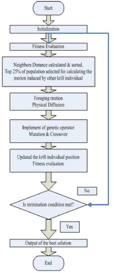
Fig.2. Flowchart of KH Algorithm with neighborhood distance concept

Table 3. Benchmark Functions

Function Name	Dimension	Type	Range	Definition	Solution
Griewank	30	Continuous, differentiable, non-separable, scalable, multimodal	[-100,100]	d x ² d x f = / --- ¹ --1 1 cos( ) + 1 j i ^x = 1 4000 i = ¹	f(x)=0
Ackley	30	Continuous, differentiable, non-separable, scalable, multimodal	[-35,35]	f = 20 + e — 20 e 7 — У D x 2 — ^J 2 D = 1 i e" D X D = i cos(2 ^x i )	f(x)=0
Booth	30	Continuous, differentiable, non-separable, non-scalable, unimodal	[-10,10]	f = ( x ^ + 2 X 2 — 7) + (2 x ^ + X 2 — 5)	f(x)=0
Rastrigin	30	Continuous, differentiable, separable, multimodal	[-5.12,5.12]	f 4 = 10 D + X DDD ( x l — 10cos(2 nx i ))	f(x)=0
Alpine	30	Continuous, Non-differentiable, separable, scalable, multimodal	[-10,10]	■^f 5 = X D x i ^Sin⁽ x i ) ⁺ 0.¹ x i	f(x)=0
Schwefel	30	Continuous, differentiable, separable, scalable, multimodal	[-500,500]	f 6 =^— X D xi ^sin -M	f(x)=- 418.983
Sphere	30	Continuous, differentiable, separable, scalable, multimodal	[-5.12,5.12]	. f 7 = X D =1 x 2	f(x)=0
Rosenbrock	30	Continuous, differentiable, non-separable, scalable, unimodal	[-2, 2]	f = X D ^—111 00 ( x ₊1— x 2 ) ² + ( x. — 1 ) ²1 .7 8 А=Ц =1 L \ i +1 i * \ 1 / J	f(x)=0

Table 4. Statistical Performance of KH variants on Benchmark Problem

Function	D	Method	N	Imax	Best fitness	Worst fitness	Mean fitness	SD	CPU Time (sec)
f 1	2	KHA	100	100	1.2309x10-2	3.8590x10-1	1.2919x10-1	2.0732x10-2	10.28
		KHAMC	100	100	1.6069x10-7	2.4664x10-3	4.3616x10-4	1.5072x10-4	10.24
		KHAMCD	100	100	4.6781x10-9	8.7742x10-4	5.1675x10-5	4.2523x10-5	7.29
	20	KHA	100	100	3.2079x10-4	2.3175x10-1	8.4477x10-2	1.7268x10-2	10.38
		KHAMC	100	100	1.7128x10-6	2.1404x10-3	3.1334x10-4	1.1908x10-4	10.37
		KHAMCD	100	100	5.2389x10-10	5.5851x10-4	5.0677x10-5	2.8277x10-5	7.37
	30	KHA	100	100	5.6578x10-4	3.8556x10-1	5.9577x10-2	1.9901x10-2	10.43
		KHAMC	100	100	2.1187x10-8	7.2481x10-3	1.0649x10-3	4.2692x10-4	10.51
		KHAMCD	100	100	3.1535x10-9	1.7069x10-3	1.4858x10-4	8.9533x10-5	7.74

Function	D	Method	N	Imax	Best fitness	Worst fitness	Mean fitness	SD	CPU Time (sec)
		Fuzzy KHA [36]	25	200	2.12x10-8	-------	1.5462x10-2	-------	-------
		Choatic KHA [32]	-------	500	-------	-------	5.6939x10-2	2.6886x10-2	-------
		Choatic KHA [33]	25	200	1.32x10-7	-------	1.44x10-2	-------	-------
		KHAL [38]	10	10000	-------	-------	4.1x10-3	6.8x10-3	-------
f 2	2	KHA	100	100	2.7450	1.2069x10+1	7.5091	6.4341x10-1	10.48
		KHAMC	100	100	1.8975x10-3	1.6410x10-1	4.9798x10-2	9.3817x10-3	10.33
		KHAMCD	100	100	2.7828x10-5	2.0834x10-2	4.0406x10-3	1.4270x10-3	7.33
	20	KHA	100	100	2.2341	1.2621x10+1	6.7996	6.0828x10-1	10.39
		KHAMC	100	100	2.9504x10-2	1.7021x10-1	7.1720x10-2	8.0913x10-3	10.44
		KHAMCD	100	100	1.2246x10-4	2.3592x10-2	3.2265x10-3	1.3799x10-3	7.23
	30	KHA	100	100	1.5591	1.5017x10+1	7.4434	8.0605x10-1	10.35
		KHAMC	100	100	5.8713x10-3	3.2497x10-1	6.8098x10-2	1.5643x10-2	10.43
		KHAMCD	100	100	1.0746x10-5	4.8179x10-2	6.7143x10-3	2.4956x10-3	7.35
		Fuzzy KHA [36]	25	200	1.119x10-4	-------	3.3439x10-1	-------	-------
		Choatic KHA [33]	25	200	1.268x10-4	-------	1.8594x10-1	-------	-------
		KHAL [38]	10	10000	-------	-------	6.523x10-1	2.323x10-1	-------
f 3	2	KHA	200	300	2.2981x10-3	2.8530x10-1	6.0273x10-2	1.4454x10-2	120.56
		KHAMC	200	300	9.7826x10-6	8.6048x10-1	7.7090x10-2	4.7057x10-2	120.81
		KHAMCD	200	300	4.2118x10-5	4.5324x10-1	4.9316x10-2	2.3785x10-2	105.88
	20	KHA	100	300	3.6026x10-4	3.1339x10-1	9.8358x10-2	2.3722x10-2	30.48
		KHAMC	100	300	1.9298x10-5	6.5852x10-1	7.5571x10-2	3.5505x10-2	30.83
		KHAMCD	100	300	8.4031x10-6	9.3225x10-1	6.4951x10-2	4.5088x10-2	21.77
f 4	2	KHA	100	100	3.3561x10-5	6.4810x10-1	8.4018x10-2	3.4771x10-2	10.23
		KHAMC	100	100	3.6062x10-6	1.0730x10-2	1.7521x10-3	5.1410x10-4	10.06
		KHAMCD	100	100	3.2963x10-7	1.7130x10-3	3.2657x10-4	9.5710x10-5	7.19
	20	KHA	100	100	1.3061x10-3	6.2422x10-1	6.8567x10-2	2.9756x10-2	10.21
		KHAMC	100	100	7.3550x10-6	3.5432x10-2	8.3993x10-3	1.9862x10-3	10.19
		KHAMCD	100	100	1.4927x10-7	1.6322x10-3	2.6607x10-4	8.5491x10-5	7.49
	30	KHA	100	100	1.1504x10-5	7.2139x10-1	9.1691x10-2	3.9918x10-2	10.45
		KHAMC	100	100	1.4198x10-4	8.1789x10-2	1.3374x10-2	4.9771x10-3	10.41
		KHAMCD	100	100	1.4273x10-5	4.1291x10-3	5.1064x10-4	2.3012x10-4	7.63
		Fuzzy KHA [36]	25	200	1.025096	-------	3.980158	-------	-------
		Choatic KHA [32]	-------	500	-------	-------	20.50905	4.3942	-------
		Choatic KHA [33]	25	200	3.072x10-2	-------	2.6523x10-1	-------	-------
		KHAL [38]	10	10000	-------	-------	9.6714	6.5899	-------
^f 5	2	KHA	100	500	5.4811x10-4	1.4929x10-1	3.3880x10-2	7.5166x10-3	50.56
		KHAMC	100	500	5.2634x10-6	4.9520x10-4	9.1777x10-5	3.0892x10-5	51.08
		KHAMCD	100	500	2.2140x10-9	9.5300x10-8	2.8705x10-8	4.7439x10-9	35.57
	20	KHA	100	500	1.8992x10-3	1.8324	1.2769x10-1	8.7695x10-2	51.33
		KHAMC	100	500	5.8783x10-1	26.097	5.5406	1.2903	51.30
		KHAMCD	100	500	1.6978x10-4	12.678	2.9513	8.6842x10-1	35.83
f 6	2	KHA	100	100	-726.68	-597.23	-661.66	8.353	10.20
		KHAMC	100	100	-837.97	-716.75	-824.78	6.152	10.28
		KHAMCD	100	100	-837.92	-717.73	-814.68	9.239	7.39
	20	KHA	100	100	-811.76	-546.68	-686.55	17.946	10.94
		KHAMC	100	100	-837.96	-715.08	-815.69	9.6001	10.70
		KHAMCD	100	100	-837.94	-599.54	-812.52	13.560	7.75
	30	KHA	100	100	-828.97	-583.27	-709.08	18.935	11.57
		KHAMC	100	100	-837.92	-712.30	-799.04	12.022	12.66
		KHAMCD	100	100	-837.91	-703.71	-809.94	10.752	7.53
		Fuzzy KHA [36]	25	200	6.38x10-4	-------	5.241x10-3	-------	-------

Function	D	Method	N	Imax	Best fitness	Worst fitness	Mean fitness	SD	CPU Time (sec)
		Choatic KHA [32]	-------	500	-------	-------	-5905.55	2361.01	-------
		Choatic KHA [33]	25	200	1.874x10-4	-------	2.2151x10-2	-------	-------
f7	2	KHA	100	100	9.3244x10-5	1.3229x10-1	1.8492x10-2	7.1446x10-3	11.72
		KHAMC	100	100	6.2953x10-8	2.2142x10-5	6.6838x10-6	1.7277x10-6	11.97
		KHAMCD	100	100	1.0547x10-10	2.2662x10-5	2.4920x10-6	1.4490x10-6	8.88
	20	KHA	100	100	8.0312x10-5	2.3803x10-2	5.2903x10-3	1.5889x10-3	12.00
		KHAMC	100	100	1.3340x10-7	4.9025x10-5	1.0330x10-5	3.1152x10-6	11.76
		KHAMCD	100	100	2.9633x10-10	1.8687x10-5	2.7952x10-6	1.0101x10-6	8.28
	30	KHA	100	100	2.8513x10-5	8.8107x10-2	9.8531x10-3	4.4336x10-3	11.49
		KHAMC	100	100	2.8175x10-7	7.2317x10-5	1.4779x10-5	4.9660x10-6	11.37
		KHAMCD	100	100	6.5458x10-12	7.4766x10-6	1.3395x10-6	4.1764x10-7	7.96
		Fuzzy KHA [36]	25	200	4.68x10-5	-------	0.000258	-------	-------
		Choatic KHA [32]	-------	500	-------	-------	0.3541	0.318221	-------
		Choatic KHA [33]	25	200	0.0195	-------	0.24187	-------	-------
		KHAL [38]	10	10000	-------	-------	0.2504	0.2135	-------
f8	2	KHA	100	100	5.3259x10-6	5.5072x10-2	5.5912x10-3	2.7019x10-3	11.77
		KHAMC	100	100	1.2777x10-2	6.3791x10-1	1.5062x10-1	3.0501x10-2	11.72
		KHAMCD	100	100	1.5709x10-2	5.9110x10-1	1.8952x10-1	3.0650x10-2	8.17
	20	KHA	100	100	1.2544x10-4	9.0696x10-2	1.8495x10-2	5.44680x10-3	11.85
		KHAMC	100	100	6.2359x10-3	3.2100x10-1	9.6901x10-2	1.7849x10-2	11.94
		KHAMCD	100	100	3.7283x10-3	5.8347x10-1	1.1992x10-1	2.8997x10-2	8.71
	30	KHA	100	100	2.7725x10-5	1.9508x10-1	4.2240x10-2	1.19939x10-2	11.76
		KHAMC	100	100	4.8975x10-3	2.8506x10-1	1.2771x10-1	1.7381x10-2	11.61
		KHAMCD	100	100	3.9030x10-3	2.3346x10-1	1.1508x10-1	1.8295x10-2	8.26
		Fuzzy KHA [36]	25	200	3.18330701	-------	7.807	-------	-------
		Choatic KHA [33]	25	200	3.983x10-5	-------	0.000165	-------	-------
		KHAL [38]	10	10000	-------	-------	0.0048	0.0108	-------

D: Dimension, SD: Standard Deviation

ш ш о Й

10Ьт

-I

np=50 np=100 np=150 np=200

5 1

Iteration

8 ,---------.---------,---------,— I- np=50

np=100

np=150

np=200

0 20 40 60 80 100

Iteration

o.s

0.6

£0.4

0.2

-0

Iteration

np=50 np=100 np=150 np=200

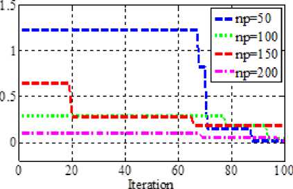
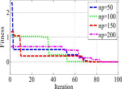
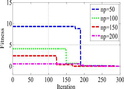
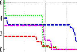
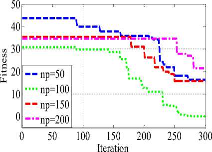
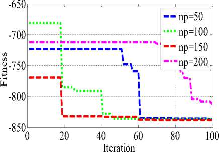
Fig.3. Convergence Characteristic of KHAMCD for different population on 20-D benchmark

C. Comparison of convergence characteristics

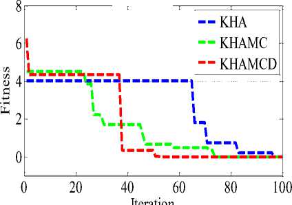
Convergence characteristic of KHAMCD algorithm are plotted with change in population in Fig 3 which shows that with increase in population the convergence improves. To make fair comparison between KHA, KHAMC and KHAMCD the convergence characteristics for different benchmark functions are compared in Fig 4, and the performance of KHAMCD is found to be better.

1.5

о fl

0.5

I I

-------------------I

Iteration

(Z) tZ)

□

I I

tZ) tZ) □ 6

KHA KHAMC KHAMCD

о fl

10L

i i

3 \-I V

KHA KHAMC KHAMCD

Iteration

KHA KHAMC KHAMCD

50 100 150 200 250 300

Iteration

KHA KHAMC KHAMCD

I I I

-500

-600

11 i '/"T -t I.

tZ) tZ) □ 6

-700

-800

50 100 150

Iteration

200 250 300

-9000

I I I

KHA

KHAMC

KHAMCD

Iteration

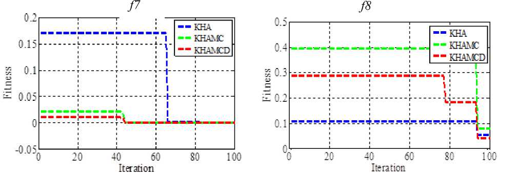
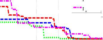
Fig.4. Comparison of convergence characteristics of variants of KHA

D. Consistency Analysis

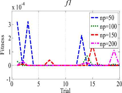
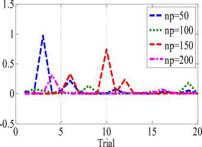
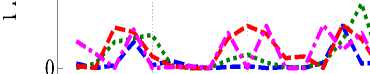
As proposed KHAMCD uses random operators similar to other stochastic search optimization technique and hence in every trial the algorithm converge to slightly different value. Therefore, it is general practice to conduct various trials and statistical analysis is also carried out on benchmark functions as shown in Table 5. Also it is illustrated using Fig 5 with different population on 20-D. It is observed that population size of 100 good consistencies compared to other population for f1 - f5, f8 whereas f6, f7 have better consistency with population size of 150 and 200.

Table 5. Consistency Analysis of KHAMCD with different population size

Function Name	N	Imax	Best fitness	Worst fitness	Mean	Standard Deviation
f1	50	100	5.2736x10-14	1.4562x10-1	2.1843x10-2	1.1627x10-2
	100	100	8.6808x10-13	3.9258x10-4	2.4350x10-5	1.9234x10-2
	150	100	1.4977x10-13	1.5364x10-4	1.0477x10-5	7.6011x10-6
	200	100	1.7531x10-10	1.0739x10-4	8.9068x10-6	5.3135x10-6
f2	50	100	1.2343x10-6	4.0871x10-2	3.2304x10-3	2.2343x10-3
	100	100	7.2152x10-7	4.5232x10-2	4.8895x10-3	2.4332x10-3
	150	100	4.8540x10-6	4.7975x10-2	5.8461x10-3	2.4157x10-3
	200	100	3.2882x10-6	3.2535x10-2	1.0839x10-2	2.4090x10-3
f3	50	300	7.8347x10-5	9.6875x10-1	7.5608x10-2	4.7113x10-2
	100	300	3.1727x10-4	1.8439x10-1	2.4747x10-2	1.0687x10-2
	150	300	1.6369x10-4	7.3522x10-1	7.0285x10-2	3.9045x10-2
	200	300	1.1243x10-4	3.1155x10-1	2.9850x10-2	1.5157x10-2
f4	50	100	1.2438x10-8	9.9565x10-1	8.0639x10-2	5.3946x10-2
	100	100	2.3078x10-7	1.8638x10-3	4.6818x10-4	1.0556x10-4
	150	100	7.4842x10-7	1.6456x10-3	2.8183x10-4	7.2329x10-5
	200	100	1.8448x10-5	1.4651x10-3	2.8534x10-4	6.6840x10-5
f5	50	500	2.5094x10-2	20.524	2.9311	1.0796
	100	500	3.3115x10-3	31.275	6.3757	1.8344
	150	500	1.3246x10-2	20.726	8.3712	1.7670
	200	500	2.9093x10-3	25.036	8.4455	1.9047
f6	50	100	-837.94	-685.33	-780.43	13.311
	100	100	-837.92	-663.17	-789.62	13.822
	150	100	-837.96	-719.13	-824.79	7.8827
	200	100	-837.93	-717.05	-818.89	9.4561
f7	50	100	7.1146x10-11	5.8820x10-5	3.6337x10-6	2.8627x10-6
	100	100	1.0717x10-10	4.2097x10-5	3.2639x10-6	2.0344x10-6
	150	100	1.6174x10-08	1.4042x10-5	3.0890x10-6	9.3391x10-7
	200	100	1.6004x10-12	5.7270x10-6	1.3783x10-6	3.8511x10-7
f8	50	100	1.9340x10-2	1.1057	0.27688	0.057311
	100	100	3.7283x10-3	0.58347	0.11992	0.028997
	150	100	4.1531x10-3	0.24786	0.097353	0.016987
	200	100	9.8037x10-3	0.19688	0.085857	0.015160

Л И и

0.1

0.05

A I I

•*»

/ A

/ \

10 Trial

np=50 np=100 np=150 np=200

Fitness Fitness

ю ю о

Е f5

0.03

0.02

0.01

-500

np=50 np=100 np=150 np=200

гл ГЛ О

-600

-700

-800

10 Trial

-9000

np=50 np=100 np=150 np=200

I I I I I I

1 п II 11

I I I I I

10 Trial

np=50 np=100 np=150 np=200

\\ /Л\/

10 Trial

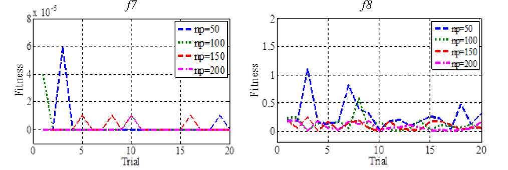
Fig.5. Consistency Analysis of KHAMCD on 20-D benchmark

IV. E CONOMIC L OAD D ISPATCH P ROBLEM

In this section KHAMCD algorithm is used to optimize practical Economic Load Dispatch (ELD) problem. ELD is key issue related with power system operation and control with goal is to find out most reliable, efficient and low cost operation of power system that can capable to match required power demand by proper dispatch of output from committed generators. ELD is complex optimization problem with main objective is to minimize the cost function and has to satisfy the operating constraints too. These types of problem have many minima and hence classical method unable to provide global best solution. On the other hand population based stochastic search NI method often provides near global solution is a better choice for solution of these types of problem.

Various optimization techniques as lamda iteration [41], quadratic programming and GAMS [52], differential evolution(DE)[43], teaching learning based optimization(TLBO)[44], Chemical Reaction

Optimization (CRO) [45], krill herd algorithm(KHA) [46,53] invasive weed optimization(IWO) [47], gravitational search (GSA)[48], flower pollination algorithm(FPA) [49], Artificial Bee Colony(ABC) [50], rooted tree optimization(RTO) [51] and hybrid DE with particle swarm optimization (PSO) [52] are successfully applied for solution of ELD problem. A comprehensive review of NI techniques for solution ELD problem is presented in [40]

To validate the performance of proposed KHAMCD it is tested on two standards complex constraint comparative medium and large scale ELD problem as below.

A. ELD formulation as cost function

The objective function corresponding to the power generation cost can be approximated as quadratic function of the active power outputs of committed the generating units. Symbolically, it is represented as:

Minimize F = У, N f ( P ) (13)

Where f ( P i ) = a i P i 2 + b i P i + C i (14)

i=1,2,3,………N ai, bi and ci represents its cost coefficients. Expression for cost function (14) corresponding to ith generating unit, Pi is the real power output (MW) and N is the number of online generator used for power dispatched. The cost function with valve point loading effect is computed as[48,49:

f ( P i ) = a , P ² + bP + c i + e x sin f , x ( P min - P i )}

Where e i and f i indicating the valve point effect of i^th generator.

Subjected to constrains as

1) Power balance constraint

N(16)

i=1 i DL

The transmission losses occurring in the system can be expressed using B-loss coefficients as [41]:

P = T N P ^B, P + Y N PB o + B oo (17)

L i=^i=1 i iJ j i=^i=1 i i000

2) Operating limit constraint

Pmin < P < Pmin, where i= 1,2,_.N(ig)

The generated output of i^th generator should lie between specified lower and upper limit.

3) Constraints due to prohibited operating zones

The prohibited operating zones (POZ) are the certain range of output power of a generator, in that rage of operation unnecessary vibration in turbine shaft takes place which may damage the shaft and bearing and hence operation is avoided in such regions. POZ makes the objective function discontinuous, therefore feasible operating zones of power generating unit can be depicted as:

P min < P < P P i

P ^x ^- ¹< P* < P ^x

P - nz / p / pmax P Gi < P Gi < P Gi

x = 2,3 nz ,^ (19)

Where, P ^x andP^x are the lower and upper operating limits of the x^th prohibited operation zone for i^th power generating unit.

B. Results and discussion

The applicability and viability of the aforementioned proposed KHAMCD algorithm for practical applications has been tested on two different test cases of ELD problem with population size (N) set at 100 and other parameter are similar as in section III.A.

1) Fifteen unit system with POZ and loss

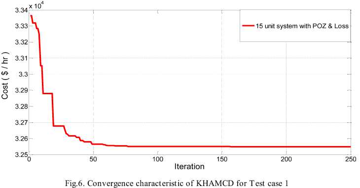
The system contains fifteen thermal generating units. Four power generating unit as 2, 5, 6 and 12 has prohibited operating zones. The fuel cost coefficient data and transmission line loss coefficient are adopted as per [46]. The total load demand on the system is 2630 MW. The optimum generation schedule obtained by proposed algorithm is presented in Table 6 and the statistical comparison of result is made in Table 7 respectively. The optimum generation cost obtained by KHAMCD 32548.0031$/hr which is found to be slightly inferior to KH IV [46], but considering overall statistical evaluation, the performance of KHAMCD is found to be better and consistent. The convergence characteristic for this test technique provides better results while satisfying the case is plotted in Fig.6. associated operating constraints.

It can be seen from results that the KHAMCD

Table 6. Optimum generation of KHAMCD for Test Case 1

Unit	KH IV [46 ]	KHAMCD	Unit	KH IV [46 ]	KHAMCD
P1	455	455	P10	31.2698	35.6215
P2	455	455	P11	76.7013	74.3593
P3	130	130	P12	80	80
P4	130	130	P13	25	25
P5	233.8017	231.7891	P14	15	15
P6	460	460	P15	15	15
P7	465	465	∑ P (MW)	2656.7728	2656.7699
P8	60	60	Ploss (MW)	26.7673	26.7699
P9	25	25	Total cost ($/h)	32547.3700	32548.0031

Table 7. Statistical results of KHAMCD for Test Case 1

Method	Min Cost($/hr)	Mean Cost($/hr)	Max Cost($/hr)	S.D	CPU time(sec)
KH IV[46 ]	32547.3700	32548.1348	32548.9326	NA	NA
DEPSO[54 ]	32588.8100	32588.9900	32591.4900	4.0200	1.9600
DPD [54]	32548.5857	32556.6793	32564.4051	2.0956	1.9800
KHAMCD	32548.0031	32548.1020	32548.354	0.1570	1.870

2) Forty unit nonconvex system

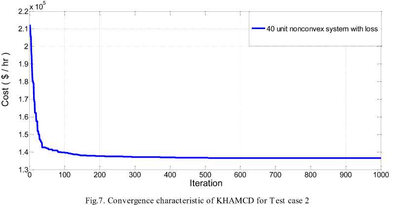
To examine the superior quality of solution and robustness of KHAMCD algorithm a more realistic test case with valve point loading effect and transmission line losses is included here. The fuel cost coefficient data and transmission line loss coefficients are adopted from [47]. The power demand for system is 10500MW. Solution in terms of optimum generation schedule obtained by simulation is presented in Table 7I. The statistical performance over twenty trials is tabulated in Table 9. The best operating cost achieved by the KHAMCD method is 136446.4053$/hr .The comparison of result has been made with hybrid genetic algorithm with ant colony optimization (GAAPI) [42], shuffled differential

evolution (SDE) [43], teaching learning based optimization (TLBO) [44], oppositional real coded chemical reaction optimization (ORCCRO) [45] , krill herd algorithm (KHA) [46], oppositional invasive weed optimization (OIWO) [47] and most recently reported Opposition-based krill herd algorithm (OKHA)[53], hybrid PSO DE approach[54]. Here it can be observed that proposed method KHAMCD is able to achieve cheapest generation cost as compared to other reported methods. Smooth and stable convergence characteristic of this system obtained by KHAMCD algorithm for power demand of 10500MW with transmission loss is shown in Fig 7.

Table 8. Optimum Generation of KHAMCD for Test Case 2

unit	KHAMCD	KH IV[46 ]	OIWO[47]	SDE [43]	unit	KHAMCD	KH IV[46 ]	OIWO[47]	SDE [43]
P1	114	114	113.9908	110.06	P21	523.2794	524.4678	549.9412	544.81
P2	114	114	114.0000	112.41	P22	535.9596	535.5799	549.9999	550
P3	120	120	119.9977	120	P23	523.2794	523.3795	523.2804	550
P4	179.7331	190	182.5131	188.72	P24	523.2794	523.15527	523.3213	528.16
P5	87.8005	88.5944	88.4227	85.91	P25	523.2794	524.1916	523.5804	524.16
P6	140	105.5166	140.0000	140	P26	523.2794	523.5453	523.5847	539.10
P7	300	300	299.9999	250.19	P27	10	10.1245	10.0086	10
P8	300	300	292.0654	290.68	P28	10	10.1815	10.0068	10.37
P9	300	300	299.8817	300	P29	10	10.0229	10.0123	10
P10	279.5997	280.6777	279.7073	282.01	P30	87.7999	87.8154	87.8664	96.10
P11	168.7998	243.5399	168.8149	180.82	P31	190	190	190.0000	185.33
P12	94	168.8017	94.0000	168.74	P32	190	190	189.9983	189.54
P13	484.0392	484.1198	484.0758	469.96	P33	190	190	190.0000	189.96
P14	484.0392	484.1662	484.0477	484.17	P34	200	200	199.9940	199.90
P15	484.0392	485.2375	484.0396	487.73	P35	200	164.9199	200.0000	196.25
P16	484.0392	485.0698	484.0886	482.30	P36	164.7999	164.9787	164.8283	185.85
P17	489.2794	489.4539	489.2813	499.64	P37	110	110	110.0000	109.72
P18	489.2794	489.3035	489.2966	411.32	P38	110	110	109.9940	110
P19	511.2794	510.7127	511.3219	510.47	P39	110	110	110.0000	95.71
P20	550	511.3040	511.3350	542.04	P40	550	512.0677	550.0000	532.43
Total cost ($/h)						136446.4053	136670.3701	136,452.677	138,157.46
P loss (MW)						958.8845	978.9251	957.2965	974.43

Table 9. Statistical results of KHAMCD for Test Case 2

Method	Min Cost($/hr)	Mean Cost($/hr)	Max Cost($/hr)	S.D	CPU time(sec)
GAAPI [42]	139864.96	NA	NA	NA	NA
SDE [43]	138,157.46	NA	NA	NA	NA
ORCCRO[45 ]	136,855.19	136,855.19	136,855.19	NA	14
TLBO[44]	137814.17	NA	NA	-------	-------
QOTLBO[44]	137329.86	NA	NA	-------	-------
OIWO [47 ]	136,452.68	136,452.68	136,452.68	NA	10.7
KHA-IV[46 ]	136670.3701	136671.2293	136671.8648	NA	NA
OKHA[53]	136,575.97	136,576.15	136,576.64	NA	NA
KHAMCD	136446.4053	136454.8868	136474.1348	11.0218	9.964

V. C ONCLUSION

Krill herd algorithm (KHA) belongs to the family of nature inspired stochastic search algorithms. To improve global search capability and convergence characteristics, the basic KHA has been improved by (i) adding crossover and mutation operators (KHAMC) and (ii) by including neighborhood distance concept (KHAMCD). The modified versions of KHA are employed to solve eight unimodal/multimodal benchmark functions as well as two non-smooth and non-convex ELD problems of power system. The basis KHA was tested on different mathematical benchmark problems and its performance was found to be satisfactory in terms of convergence and consistency. The performance of the algorithm was found to be improved in terms of solution quality by using mutation and crossover operators. When neighborhood distance concept was added, for the same accuracy, the computational time was reduced to around 26 to 30% and exploration and exploitation level of krill herd is balanced properly. Various trials were conducted with different initial populations and it was found that every time KHAMCD produced accurate results within tolerance band. As compared to recently reported results in literature, the performance of KHAMCD is found to better in terms of solution quality. From this comparative analysis, it can be concluded that the proposed methodology can effectively be used to solve smooth as well as non-smooth constrained optimization problems.

Список литературы Improved Krill Herd Algorithm with Neighborhood Distance Concept for Optimization

Holland J H. Genetic algorithms and the optimal allocation of trials. SIAM J. Comput., 1973, 2(2): 88-105.
Beyer H G, Schwefel H P. Evolution Strategies: A Comprehensive Introduction. Journal Natural Computing, 2002, 1 (1): 3–52.
Fogel L J, Owens A J, Walsh M J. Artificial intelligence through simulated evolution. 1966, Wiley, New York.
Reynolds R G. An introduction to cultural algorithms. In Proceedings of the 3rd annual conference on evolutionary programming, 1994. 131–139.
Kirkpatrick S, Gelatt C D, Vecchi M P. Optimization by simulated annealing. Science, 1983, 220(4598):671–680.
Glover F. Tabu search. Part I. ORSA Journal on Computing, 1989, 1(3):190–206.
Kennedy J, Eberhart R C. Particle swarm optimization. In Proceedings of IEEE international conference on neural networks, Piscataway, NJ, 1995. 1942–1948.
Dorigo M, Maniezzo V, Colorni A. The ant system: optimization by a colony of cooperating agents. IEEE Trans. Syst. Man Cybern. Part B: Cybern., 1996, 26:29–41.
Geem Z W, Kim J H, Loganathan G. A new heuristic optimization algorithm: harmony search. Simulation, 2001,76(2): 60–68.
Ocenasek J, Schwarz J. Estimation of distribution algorithm for mixed continuous-discrete optimization problems. In 2nd Euro-International Symposium on Computational Intelligence, 2002. 227–232.
Passino K M. Biomimicry of bacterial foraging for distributed optimization and control. IEEE Control Syst. Mag., 2002, 22(3): 52–67.
Haddad O B, Afshar A, Marin o M A. Honey bees mating optimization algorithm (HBMO): a new heuristic approach for engineering optimization. Proceeding of the First International Conference on Modeling, Simulation and Applied Optimization, 2005.
Shah-Hosseini H. The intelligent water drops algorithm: A nature-inspired swarm-based optimization algorithm. International Journal of Bio-Inspired Computation, 2009, 1(1/2): 71–79.
Yang X-S. Firefly algorithms for multimodal optimization. Stochastic Algorithms, Foundations and Applications. Springer, 2009. 169–178.
Karaboga D, Basturk B. A powerful and efficient algorithm for numerical function optimization: artificial bee colony (ABC) algorithm. J Glob Optim, 2007, 39: 459-471.
Rashedi E, N-pour H, Saryazdi S. GSA: A Gravitational search algorithm. Information Sciences, 2009, 179: 2232-2248.
Yang X-S. A new metaheuristic bat-inspired algorithm. In J. R. Gonzalez et al. (Eds.), Nature inspired cooperative strategies for optimization (NISCO 2010). Studies in computational intelligence, Berlin:. Springer. 2010, 284: 65–74.
Rajabioun R. Cuckoo optimization algorithm. Applied Sof Computing, 2011,11: 5508-5518.
Gandomi A H, Alavi A H. Krill Herd: A New Bio-Inspired Optimization Algorithm. Communications In Nonlinear Science And Numerical Simulation, 2012, 17: 4831–4845.
Cuevas E, Cienfuegos M. A new algorithm inspired in the behavior of the social-spider for constrained optimization. Expert Systems with Applications, 2014, 41: 412-425.
Civicioglu P. Backtracking search optimization algorithm for numerical optimization problems. Applied Mathematics and computation, 2013, 219(15): 8121-8144.
Mirjalili S, Mirjalili S M, Lewis A. Grey Wolf Optimizer. Advances in Engineering Software, 2014, 69: 46-61.
Cheng M-Y, Prayogo D. Symbiotic Organism Search: A metaheuristic optimization algorithm. Computers and Structures, 2014, 139: 98-112.
Yazdani M, Jolai F. Lion optimization algorithm. Journal of Computational Design and Engineering, 2015, doi:10.1016/j.jcde.2015.06.003
Salimi H. Stochastic Fractal search: a powerful metaheuristic algorithm. Knowledge based systems, 2015, 75: 1-18.
Shareef H, Ibrahim A A, Mutlag A H. Lightning search algorithm[J]. Applied Soft Computing, 2015, 36: 315-333.
Wolpert D H, Macready W G. No free lunch theorems for optimization . IEEE Trans. Evol. Comput., 1997, 1 (1): 67–82,1997.
Marr J W S. The natural history and geography of the Antarctic krill (Euphausia superba Dana). Disc Rep, 1962, 32:33–464.
Wang G-G, Deb S, Gandomi A H, Alavi A H. Opposition based krill herd algorithm with Cauchy mutation and position clamping. Neurocomputing, 2015, dx.doi.org/10.1016.
Nikbakht H, Mirvaziri H. A new clustering approach on K-means and krill herd algorithm. 23rd Iranian conference on Electrical Engineering, 2015. 662-667.
Pandey S, Patidar R, George N V. Design of a krill herd algorithm based adaptive channel equalizer. International Symposium on Intelligent Signal Processing and Communication System, 2014. 257-260.
Saremi S, Mirjalili S M, Mirjalili S. Chaotic Krill Herd Optimization Algorithm. Procedia Technology, 2014, 12: 180-185.
Bidar M, Fattahi E, Kanan H R. Modified krill herd optimization algorithm using chaotic parameters. 4th International Conference on Computer and Knowledge Engineering, 2014. 420-424.
Wang G-G, Gandomi A H, Alavi A H. Stud krill herd algorithm. Neurocomputing, 2014, 128: 363-370.
Wang G-G, Gandomi A H, Alavi A H. An effective krill herd algorithm with migration operator in biogeography-based optimization. Applied Mathematical Modeling, 2014, 38: 2454-2462.
Fattahi E, Bidar M, Kanan H R. Fuzzy krill herd optimization algorithm. IEEE first International Conference on Networks and Soft Computing, 2014. 423-426.
Rodrigues D, Pereira L A M, Papa P J, Weber S A T. A Binary krill herd approach for feature selection. 22nd International Conference on Pattern Recognition, 2014. 1407-1412.
Li J, Tang Y, Hua C, Guan X. An improved krill algorithm: Krill herd with linear decreasing step. Applied Mathematics and Computation, 2014, 234: 356-367.
Jamil M, Yang X-S. A literature survey of benchmark functions for global optimization problems. Int. Journal of Mathematical Modeling and numerical optimization, 2013, 4: 150-194.
Dubey H M, Panigrahi B K, Pandit M. Bio-inspired optimization for economic load dispatch: a review, International Journal of Bio-Inspired Computation 2014, 6 (1), 7-21.
Wood A J, Wallenberg B F. Power Generation, Operation and Control. 1984, New York: Wiley.
Ciornei I, Kyriakides E. A GA-API Solution for the Economic Dispatch of Generation in Power System Operation. IEEE Trans Power Syst., 2012, 27 (1).
Reddy A S, Vaisakh K. Shuffled differential evolution for large scale economic dispatch. Electric Power Systems Research, 2013, 96: 237-45, .
Roy P K, Bhui S. Multi-objective quasi-oppositional teaching learning based optimization for economic emission load dispatch problem. Int. J. Electr. Power Energy Syst., 2013, 53: 937–48.
Bhattacharjee K, Bhattacharya A, Halder nee Dey S. Oppositional Real Coded Chemical Reaction Optimization for different economic dispatch problems. Electrical Power and Energy Systems, 2014, 55: 378–391.
Mandal B, Roy P K, Mandal S. Economic load dispatch using krill herd algorithm. Electrical Power and Energy Systems, 2014, 57: 1–10.
Barisal A K, Prusty R C. Large scale economic dispatch of power systems using oppositional invasive weed optimization. Applied Soft Computing, 2015, 29: 122–137.
Dubey H M, Pandit M, Panigrahi B K, Udgir M. Economic load dispatch by hybrid swarm intelligence based gravitational search algorithm. I J Intelligent Systems and Applications, 2013, 5(8): 21–32.
Dubey H M, Pandit M, Panigrahi B K. A biologically inspired modified flower pollination algorithm for solving economic dispatch problems in modern power systems. Cognitive Computation, 2015, 7(5): 594-608.
Mahdad B, Srairi K.. Solving Practical Economic Dispatch Problems Using Improved Artificial Bee Colony Method. I.J. Intelligent Systems and Applications, 2014, 07(6): 36-43.
Labbi Y, Attous D B, Gabbar H A, Mahdad B, Zidan A. A new rooted tree optimization algorithm for economic dispatch with valve-point effect. Electrical Power and Energy Systems 79 (2016) 298–311.
D. Bisen, H. M. Dubey, M. Pandit, B.K. Panigrahi, solution of large scale economic load dispatch problem using quadratic programming and GAMS: A comparative analysis, Journal of Information and Computing science, vol. 7,no.3,pp.200-2011,2012.
Ali Bulbul S M, Pradhan M, Roy P K, T. Pal. Opposition-based krill herd algorithm applied to economic load dispatch problem. Ain Shams Engineering Journal, .doi.org/10.1016/j.asej.2016.02.003
Parouha R P, Das K N. A novel hybrid optimizer for solving Economic Load Dispatch problem. Electrical Power and Energy Systems, 2016, 78:108–126.
Singh G P, .Singh A. Comparative Study of Krill Herd, Firefly and Cuckoo Search Algorithms for Unimodal and Multimodal Optimization. I.J. Intelligent Systems and Applications, 2014, 03:35-49

Еще

Статья научная