Influences of the Front Wheel Steering Angle on Vehicle Handling and Stability and a Control Theory of Steady-state

Published Online June 2011 in MECS

VHS is one of the main performances that not only affects the ease of driving but also determines the automotive safe driving on high speed. With the improvement of the road, it is paid more attention increasingly and becomes one of the most important performances of the modern car.

Early in the 1930s, people have begun to study VHS systematically. Now with the rapid development of computer technology, people make theoretical study and simulation in-depth on various factors that influence the VHS [1, 2, 3, 4 ]. Choosing a 2-DOF model of a car as the reference model to analyze the VHS, we first establish the car’s differential equations of motion, and then derive and transform the equations to obtain the relevant steady-state volume and transient volume, finally analyze the steady-state response and transient response of the vehicle. In the previous analysis, FWSA is considered small that it is simplified when we derive equations (sin§ = §,cos§ = 1 ). So it is easier to get the car’s steering sensitivity and transient yaw rate. But in reality FWSA is changing from 0° to 45°. If we do the same simplify, the results we get may be inaccurate.

In this paper, the car’s differential equations of motion are derived and solved to get the expression of the steering sensitivity and the differential equation which contains transient yaw rate and sideslip angle of the center of mass without simplifying the FWSA. We solve the equations, get the natural frequency range of transient yaw rate through its Fourier transform and plot the relevant images with matlab software. Finally we determine how the FWSA influences the level of the VHS by analyzing and comparing the images with the simplified ones. And then in order to improve the performance of the steady-state we put forward a control theory that optimizes the vehicle's performance.

• II.    LINEAR TWO DEGREES OF FREEDOM VEHICLE MODEL

• A.    Modeling

In this paper, we choose the linear 2-DOF vehicle model as a reference model[5]. It is shown in Fig. 1.

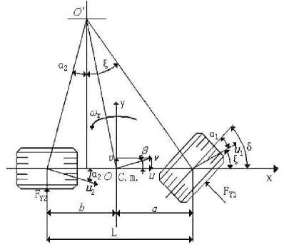
Figure 1. Two degrees of freedom vehicle model.

FY1 and FY2 are the lateral forces due to the contact between the tyre and and the road surface at each front and rear wheel. 5 is the front wheel steering angle. u 1 and u2 are the velocities of each front and rear axle’s midpoint. a1 and a2 are sideslip angles of the front and rear wheel. p = uju is the sideslip angle of the center of mass. £ is the angle between u 1 and x -axis.

• B.    Establishing Motion Differential Equation of the 2-DOF Vehicle Model

Make the origin of the vehicle coordinate system coincides with the vehicle mass center. Mass distribution parameter of the vehicle is a constant relative to the car’s moving coordinate system. From the Fig. 2, we can obtain the oy -axis’s variation of velocity component as follow.

(u + Au)cosA9 - и + (u + Au)sinA9 = и cos A 9 + Au cos A 9 - и + u sin A9 + Au sin A 9

As A 9 is small and the second order trace can be ignored, the formula above becomes Au - u A9 . Then we can get the oy -axis’s absolute acceleration component of the center of mass as follow:

a y = U + u a _r                 (1)

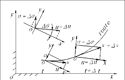
Figure 2. Analysis chart of vehicle movement.

Beacause

F Y 1 = k 1 a 1 ,F Y 2 = k ₂ a ₂ , § = ( u + a a _r )/ u = p + a aj u , and a 1 = - ( 5 - ^ ), a ₂ = ( u - b a r )/ u , the motion differential equation of the two degrees of freedom(2-DOF) vehicle is as follow.

If the FWSA is simplified, the motion differential equation of the vehicle is:

( k 1 + k ₂ ) p +— ( ak 1 - bk ₂ ) a _r - k 1 5 = m ( & + u a _r )    (3)

( ak 1 - bk ₂ ) p +— ( a²k 1 + b ² k ₂ ) a _r - ak 1 5 = I_Z< h .

If the FWSA is not simplified, the motion differential equation of the vehicle is:

( k 1 cos 5 + k ₂ ) p +— ( ak 1 cos 5 - bk ₂ ) a _r

• -    k 1 5 cos 5 = m ( z & + u a r )                     (4)

( ak 1 cos 5 - bk ₂ ) p + — ( a ² k 1 cos 5 + b ² k ₂ )a_r

и

• -    ak 1 5 cos 5 = I_Z & _r

Equation (3) and (4) are the two cases that we need to study. Finally we analyze the steady-state’s characteristics and put forward a control theory on the basis of the latter situation.

• III. STEADY - STATE RESPONSE , TRANSIENT RESPONSE AND THE AMPLITUDE - FREQUENCY CHARACTERISTIC OF YAW VELOCITY

In this paper, the relevant parameters of the 2-DOF vehicle model are as follow:

m = 1818.2 kg, L = 3.048m,     a = 1.463m, b = 1.585m, k1 =-62618N / rad,             k 2 =-110185 N / rad,

I_z = 3885 kg • m ²

• A.    Steady-state Response

In the steady state, a _r = C , U = 0, a . = 0 , (4) is changed into the following form:

( k 1 cos 5 + k 2 ) ^U +— ( ak 1 cos 5 - bk ₂ ) a _r u u

• -    k 1 5 cos 5 = mu a _r                        (5)

( ak 1 cos 5 - bk ₂ ) ^U + — ( a² k 1 cos 5 + b ² k ₂ ) a _r u u

• -    ak 1 5 cos 5 = 0

Using (5), we can obtain the steering sensitivity as follow:

k 1 cos 5в + a ^- - 5 ) + k 2 fp - ^2) )

V u ) V u ) = m ( U + u ® r )

ak 1 cos j f p + a ^- - 5 ) - bk ₂ f p - b ^-

V u ) V u , = I z & .

Where I_Z is the moment of inertia of the vehicle body with respect to the vertical axis, z . a r is the yaw angular acceleration of the vehicle.

^a r ) 5 )

s

u

L

, m I a

1 + -?l —

L ² V k ₂

b )

------------I u k 1 cos 5 )

Let K denote m_ I A - ^b

L ² V k ₂    k 1 cos 5

Obviously K

changes along with 5 . Because u and 5 are all variables, we first determine the value of 5 , then plot the relation curves of steering sensitivity changing follow the velocity of the vehicle under different 5 and compare

with the situation that 5 is not simplified. The curves are shown in Fig. 3 and Fig. 4.

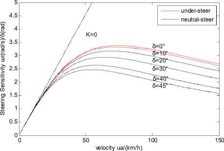
Figure 3. Relationship between steering sensitivity and velocity when FWAS changes from 0 ° to 45 °

• B.    Transient Response

Owing to в = —, we obtain the following equation u from (4).

^r _

• -1-    ( k 1 cos 5 + k 2 ) —Ц- ( ak 1 cos 5 - bk 2 - mu ² ) ⁽⁷⁾ mu             mu ²

— ( ak_v cos 5 - bk₂ )    —"—( a 2 k_v cos 5 + b ² k₂ )

. I/                    Izux                    J

•

в

. dr

^^^^^^B

---k 1o cos о mu

— ak, 5 cos 5

I z ¹

When front wheel angle step input, the mathematical expression for the FWSA is:

t < 0,5 = 0 '

t > 0,5 = 5o > t > 0,5 = 0

Change the value of 5 ₀ , transient yaw rate can be obtained under different front-wheel angle.

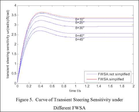
Here let u = 20 m / s and change the value of 5 ₀ , we use the ode45 solver to solve the differential equations above, obtain the transient analytical solutions of transient yaw rate and sideslip angle of the center of mass and plot the images shown in Fig. 5 and Fig. 6 in matlab.

/в = —— ( k 1 cos 5 + k 2 ) в

mu

+—Ц-(ak 1 cos 5 - bk2 - mu2 )®r ——k 15cos 5 mu2

• <

A r = — ( ak 1 cos 5 - bk 2 ) в

• 1    Iz1

+-- ( a ² k , cos 5 + b ² k₂ d--ak_x 5 cos 5

I Izu'I

Equation (6) is written in matrix form as follow:

• C.    Amplitude-frequency Characteristic of the Transient Yaw Rate under Different FWSA

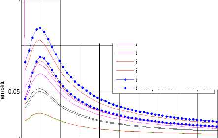
The transient yaw rate is changed into the fast Fourier transform form in matlab. Then we can obtain its amplitude-frequency characteristic curve shown in Fig. 7.

δ=10° δ=10° δ=20° δ=20° δ=30° δ=30° δ=40°

δ=40° δ=45° δ=45°

0.15

0.1

0 0

frequency (Hz)

Figure 7. Amplitude-frequency Characteristic Curve of

The Transient Yaw Rate under Different FWSA.

FWSA:not simplified FWSA: simplified FWSA:not simplified FWSA: simplified FWSA:not simplified FWSA: simplified FWSA:not simplified

FWSA: simplified FWSA:not simplified FWSA: simplified

• IV.    C OMPARATIVE ANALYSIS OF THE IMAGES

• A.    Steady-state Steering Sensitivity under Different FWSA

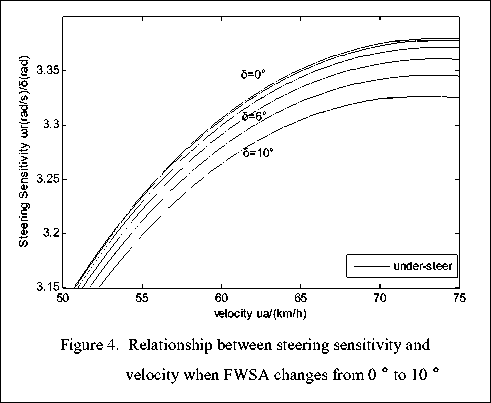
From the Fig. 3 and Fig. 4 we can see that the curves change very little when the FWSA changing between 0° and 10°( 5 = 0 ° means that the FWSA is simplified.). They begin to change significantly after 10°. With the increase of the FWSA, the vehicle’s steering sensitivity curve approaches the x-axis gradually and the vehicle’s understeer increases, but the characteristic speed of the vehicle decreases. When the FWSA is fixed and the vehicle’s speed is relatively low, the curve of the steering sensitivity is close to that in the neutral-steer state(K=0). That is to say the vehicle in low speed can be seen in the neutral-steer state. The steering sensitivity first increases, reaching a maximum value, and then begins to decrease with the increase of the speed. We can see that the vehicle has a clear under-steer characteristics. When u a = 75 km / h , the relative error of the steering sensitivities which are obtained when 5 = 0 ° and 5 = 10 ° is about 2%. When 5 = 0 ° and 5 = 45 ° , the relative error is about 51%. So when FWSA is small, it has a little influence on the steering sensitivity. But when it becomes large, it has a great impact on the steering sensitivity. Then we can draw a conclution that when FWSA is large the influence on the VHS can not be ignored.

• B.    Transient Steering Sensitivity and Sideslip Angle under Different FWSA

As shown in Fig. 5, the transient steering sensitivity curve is only one when simplifying FWSA. when FWSA is not simplified, the transient steering sensitivity decreases and decreases at a faster pace with the increase of the FWSA. The transient steering sensitivity first increases, then begin to decrease to a stable value and reach steady state at last with the time increasing when FWSA is fixed. When t = 2s , the relative error of the transient steering sensitivities which are obtained when 5 = 10° and FWSA simplified is about 1%. The relative error between 5 = 45° and FWSA simplified reaches up to 42%. So according to the analysis, we can see that the large FWSA has an oversized impact on the transient steering sensitivity.

The following we analyze how the variational FWSA affects the side slip angle of the center of mass which is also an important aspect of the evaluation of VHS and can be used to describe the vehicle’s trajectory problem. + в indicates that the radius of the vehicle’s actual trajectory is shorter than that of the vehicle’s ideal trajectory while - в indicates the opposite meaning. when в is close to zero, the vehicle has the best VHS. when в doesn’t equal zero, the VHS is affected to a certain extent [6].

It can be seen from the Fig. 6 that the trends of the sideslip angle curves of the two cases are mainly the same. With the increasing of the time the curve first increases from zero to a maximum, then decreases to a negative maximum and finally stabilizes at a negative value that will not change. From the perspective of the vehicle’s trajectory, the radius of the trajectory first shortens from the ideal radius to a certain extent, then starts to increase to the ideal radius and finally stabilizes at a radius that is longer than the ideal one.

As the FWSA increases, the amplitude of variation of в increases. the gap between the largest positive value and the largest negative one is getting bigger and bigger and the value of в has the same variation under the two cases. When t = 2 s , 5 = 10 ° , the gap of в between the two cases is small. When t = 2 s , 5 = 45 ° , the gap reaches maximum and the relative error is about 28.57%.

• C.    Amplitude-frequency Characteristic of the Transient Yaw Rate under Different FWSA

From Fig. 7, we can obviously see that when f = 1Hz the yaw rate has the maximum amplitude which is the natural frequency of the vehicle. No matter how FWSA changes , the natural frequency is stabilized at around 1Hz. With the FWSA increasing the gap of the amplitude between the two cases is growing. when FWSA is small, the relative error is relatively small. But when f = 1Hz, 5 = 45 ° , the relative error is relatively large, about 63%.

• V.    AN ACTIVE CONTROL ON STEADY - STATE

• A.    the Establishment of the Control Model and Differernial Equation

As shown in Fig. 8, we add an active moment, M = c to r , to the linear 2-DOF vehicle model which is in the opposite direction of the yaw rate.

the motion differential equation of this system is as follow.

( k 1 cos 5 + k ₂ ) в + — ( ak 1 cos 5 - bk ₂ ) ® _r u

• -    k 15 cos 5 = m (— + utor)

c rn r + ( ak 1 cos 5 - bk ₂ ) в + — ( a ² k 1 cos 5 + b ² k ₂ ) ®, u

r

- ak 1 5 cos 5 = I z to .

In the steady state, to r = C , — = 0, to r = 0 , (8) is changed into the following form:

( k 1 cos 5 + k ₂ ) ^— + — ( ak 1 cos 5 - bk ₂ ) ® _r

u u

• -    k 1 5 cos 5 = mu to r

( ak 1 cos 5 - bk ₂ ) ^— + — ( a ² k 1 cos 5 + b ² k ₂ + cu to r u u

• -    ak 1 5 cos 5 = 0

  
  
  
  
  

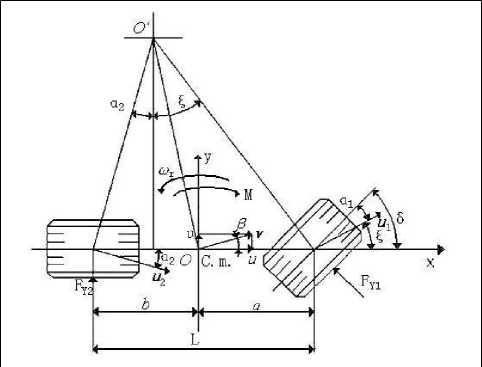
  Figure 8. the Vehicle Model Added Control Moment.

  
  

• B.    Analysis of the Steady-state Response with the Coefficient c

Using (9), we can obtain the steering sensitivity of the steady-state as follow:

u tor j =/L(10)

• ⁵    J. _л mu ² f a b j cu f 1       1

^$ 1 +                        | +               +

L ² ( k ₂ k ₁ cos 5 J L ² ( k ₁ cos 5 k ₂

In (10), u , c , 5 are variables. So we first determine the values of 5 , c and then draw the curves of the steering sensitivity changing with the velocity u , shown in Fig. 9. To make the picture clear and easy to analyze, we use only part of the value of c .

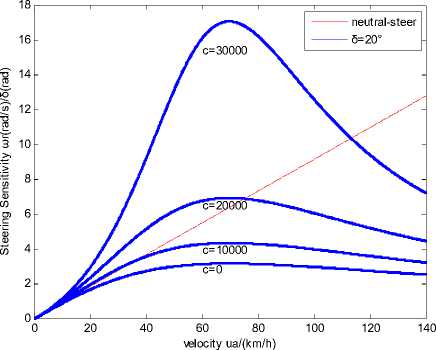
Figure 9. Relationship between Steering Sensitivity and Velocity When δ =20° , c=0~30000.

From the Fig. 9 we can draw that when c = 0 (the situation that is not under the active control), the steadystate response of the vehicle tends to neutral-steer in the low speed and begins to tend to under-steer with the increase of the speed that makes the VHS get worse. In the figure we can also see that the vehicle’s yaw rate gain of the steady-state is changing under different value of c .

C. Control Strategy

c is a controllable value. In order to improve the VHS, we can change the value of c according to the variable speed of the vehicle to adjust the vehicle's steady-state response and make it in the neutral-steer state. So we need to make the denominator of (10) equal 1. That is shown in the following.

mu2 f a b j cu f 11

2“l 1—1----^l+ rl 1^

L ^ k ₂ k ₁ cos 5 J L ^ k ₁ cos 5 k ₂

It can be changed into the following eqution.

mu ² f a "IT I k 2

b j cu f 11

------------------I + 1--+-- k 1cos5J L (k 1 cos 5 k2

From (11) we can gain that:

ak, cos 5 - bk., c = - mu----------- k 1 cos 5 + k 2

= 0 (11)

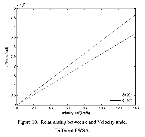
From the above equation we know that when 5 is determined, the relationship between c and the velocity is linear which is shown in Fig. 10.

From Fig. 10 we can see that the slope of the curve increases with the increasing of FWSA. That is to say the value of c increases with the FWSA increasing under the same velocity. So we can choose the appropriate value of c to make the vehicle in the best steady-state only if we know the FWSA and velocity of the vehicle.

To this end, we can install an electric device which can produce torque in the front wheel steering shaft. In order to guarantee M = ctor, we need to track the value of FWSA with an angle sensor and to track the values of velocity and yaw rate with velocity sensors. Finally the value of M is determined according to the measured values and the vehicle can be controlled.

W . CONCLUDING REMARKS

• 1)    In this paper, motion differential equation of the 2-DOF vehicle is established based on the linear two degrees of freedom vehicle model and is derived without simplifying the FWSA, then we analyze the vehicle's steady-state response, transient response and the amplitude-frequency characteristic of yaw velocity under different FWSA with the help of the software. At last we put forward a control theory that can optimize the vehicle's steady-state performance.

• 2)    The results showed that: when the FWSA is small, the steady-state response, transient response and the yaw rate of the amplitude-frequency characteristic of the both cases that the angle is simplified and not simplified don’t change much. In other word, the FWSA havs less impact on VHS. But when the angle is increasing to10°or greater, its influence on VHS is becoming apparently. Then obviously the simplified treatment will cause great error. The control theory can make the vehicle in the best steady-state.

• 3)    This article provides an accurate theoretical study on future VHS and has some reference value. The implementation of control strategie and simulation need to be further improved.

A CKNOWLEDGMENT

We would like to thank the editor and the reviews for their consideration. We also acknowledge the support by the National Natural Science Foundation of Shandong Province under the Grant 2R200PFL016 .

• [1]    Keiji Watanabe, Masanori Kitano and Akihiro Fugishima, Handling and Stability Performance of Four-track Steering Vehicles, Journal of Terramechanics, Volume 32, Issue 6, November 1995, pp. 285-302

• [2]    Hans B. Pacejka, Tyre Characteristics and Vehicle Handling and Stability, Tyre and Vehicle Dynamics (Second Edition), 2006, Pages 1-60

• [3]    Yin Niandong, Progress of Vehicle Handling and Stability, Journal of Huangshi Polytechnic College, Vol.20, No.4, Aug 2004.

• [4]    Liu Li, Chu Jiangwei and Shi Shuming, etc, Influences of the Vehicle Longitudinal Acceleration on Vehicle Handling and Stability, Journal of Vibration and Shock, Jun 2009.

• [5]    Yu Zhisheng, Automotive Theory(fourth Edition), China Machine Press, pp. 144~161.

• [6]    Zhou Hongni and Tao Jianmin, Influences of Sideslip Angle and Yaw Rate on Vehicle Handling and Stability, Journal of Hubei Automotive Industries Institute, Vol.22, No.2.

Chuan-Bo Ren, born in Weifang of Shandong province, China in 1964.5, received the Bachelor's Degree in Manufacturing from Shandong College of Agricultural Mechanization, China in 1984, the Master degree in solid mechanics from Jiangsu University of Science and Technology in 1989 and the Doctor’s degree in Structural Mechanics from Dalian University of Technology in 1998. His research interests are vehicle system dynamics, electric vehicle technology, simulation and testing of engineering structure.

He served as associate professor, professor in School of Vehicle and School of Resource and Environment, Shandong Institute of Engineering in 1997-2001, as professor in School of Traffic and Vehicle Engineering, Shandong University of Technology from 2001. He has published more than 50 papers, for example, An Implementation of Element Free-Time Precision Integration Method to Solve the 2-D Structural Vibration. Dynamics of Continuous, Discrete and Impulsive Systems. 2007 Vol. 14(S5), Solution for Dynamics Equations of Control Systems with Time-Delay by Precise Integral Algorithm, ISDA 2006, 2006.8, etc.

Prof. Ren is the permanent member of the Society of Automotive Engineers of Shandong, China and the permanent member of the Society of Theoretical and Applied Mechanics of Shandong, China. He has won the National Scientific and Technological Progress Award and National Invention Award in 2006, the Scientific and Technological Progress Award granted by the Ministry of Education of China, the Outstanding Contributions to Middle-aged and Young Expert Award of Shandong province in 2007, the Scientific and Technological Progress Award granted by Shandong Province of China, the Top Ten Science and Technology Achievement Award granted by Shandong Province of China in 2002, the Scientific and Technological Progress of Zibo Award and the Sixth Youth Science and Technology of Zibo Award. Prof. Ren has completed 11 scientific research projects, and is now carrying out 3 provincial projects.