Intelligent Adaptive Gain Backstepping Technique

Published Online January 2015 in MECS

• I.    Introduction and Background

In modern usage, the word of control has many meanings, this word is usually taken to mean regulate, direct or command. The word feedback plays a vital role in the advance engineering and science. There are several methods for controlling a robot manipulator, which all of them follow two common goals, namely, hardware/software implementation and acceptable performance. However, the mechanical design of robot manipulator is very important to select the best controller but in general two types schemes can be presented, namely, a joint space control schemes and an operation space control schemes[1]. Joint space and operational space control are closed loop controllers which they have been used to provide robustness and rejection of disturbance effect. The main target in joint space controller is to design a feedback controller which the actual motion ( qa(t) ) and desired motion ( qd(t) ) as closely as possible. This control problem is classified into two main groups. Firstly, transformation the desired motion Xd(t) to joint variable qd(t) by inverse kinematics of robot manipulators[2]. This control include simple PD control, PID control, inverse dynamic control, Lyapunov-based control, and passivity based control that explained them in the following section. The main target in operational space controller is to design a feedback controller to allow the actual end-effector motion Xa(t)

to track the desired endeffector motion X d (t) . This control methodology requires a greater algorithmic complexity and the inverse kinematics used in the feedback control loop. Direct measurement of operational space variables are very expensive that caused to limitation used of this controller in industrial robot manipulators[3]. One of the simplest ways to analysis control of multiple DOF robot manipulators are analyzed each joint separately such as SISO systems and design an independent joint controller for each joint. In this controller, inputs only depends on the velocity and displacement of the corresponding joint and the other parameters between joints such as coupling presented by disturbance input. Joint space controller has many advantages such as one type controllers design for all joints with the same formulation, low cost hardware, and simple structure.

A nonlinear methodology is used for nonlinear uncertain systems (e.g., robot manipulators) to have an acceptable performance. These controllers divided into six groups, namely, feedback linearization (computed-torque control), passivity-based control, sliding mode control (variable structure control), artificial intelligence control, backstepping control and adaptive control[4-5]. In control theory, backstepping is a technique developed circa 1990 by Petar V. Kokotovic and others for designing stabilizing controls for a special class of nonlinear dynamical systems. These systems are built from subsystems that radiate out from an irreducible subsystem that can be stabilized using some other method. Because of this recursive structure, the designer can start the design process at the known-stable system and "back out" new controllers that progressively stabilize each outer subsystem. The process terminates when the final external control is reached. Hence, this process is known as backstepping. Backstepping control is work based on cancelling decoupling and nonlinear terms of dynamics formulation of each link. This method computes the required arm torques using the nonlinear feedback control law [6-7].

In recent years, artificial intelligence theory has been used in sliding mode control systems. Neural network, fuzzy logic, and neuro-fuzzy are synergically combined with nonlinear classical controller and used in nonlinear, time variant, and uncertainty plant (e.g., robot manipulator). Fuzzy logic controller (FLC) is one of the most important applications of fuzzy logic theory. This controller can be used to control nonlinear, uncertain, and noisy systems. This method is free of some model-based techniques as in classical controllers. As mentioned that fuzzy logic application is not only limited to the modelling of nonlinear systems [13-14]but also this method can help engineers to design easier controller. Control robot arm manipulators using classical controllers are based on manipulator dynamic model. These controllers often have many problems for modelling. Conventional controllers require accurate information of dynamic model of robot manipulator, but these models are multi-input, multi-output and non-linear and calculate accurate model can be very difficult. When the system model is unknown or when it is known but complicated, it is difficult or impossible to use classical mathematics to process this model[8-9]. The main reasons to use fuzzy logic technology are able to give approximate recommended solution for unclear and complicated systems to easy understanding and flexible. Fuzzy logic provides a method which is able to model a controller for nonlinear plant with a set of IF-THEN rules, or it can identify the control actions and describe them by using fuzzy rules. It should be mentioned that application of fuzzy logic is not limited to a system that’s difficult for modeling, but it can be used in clear systems that have complicated mathematics models because most of the time it can be shortened in design but there is no high quality design just sometimes we can find design with high quality. Besides using fuzzy logic in the main controller of a control loop, it can be used to design adaptive control, tuning parameters, working in a parallel with the classical and non classical control method [9]. The applications of artificial intelligence such as neural networks and fuzzy logic in modelling and control are significantly growing especially in recent years. For instance, the applications of artificial intelligence, neural networks and fuzzy logic, on robot arm control have reported in [9].

Research about mechanical parts and control methodologies in robotic system is shown; the mechanical design, type of actuators, and type of systems drive play important roles to have the best performance controller. More over types of kinematics chain, i.e., serial Vs. parallel manipulators, and types of connection between link and join actuators, i.e., highly geared systems Vs. direct-drive systems are played important roles to select and design the best acceptable performance controllers[10-11]. A serial link continuum robot is a sequence of joints and links which begins with a base frame and ends with an end-effector. This type of robot manipulators, comparing with the load capacitance is more weightily because each link must be supported the weights of all next links and actuators between the present link and end-effector[12-13]. Serial continuum robot manipulators have been used in medical application, and also in research laboratories. One of the most important classifications in controlling the robot manipulator is how the links have connected to the actuators. This classification divides into two main groups: highly geared (e.g., 200 to 1) and direct drive (e.g., 1 to 1). High gear ratios reduce the nonlinear coupling dynamic parameters in robot manipulator. In this case, each joint is modeled the same as SISO systems. In high gear robot manipulators which generally are used in industry, the couplings are modeled as a disturbance for SISO systems. Direct drive increases the coupling of nonlinear dynamic parameters of robot manipulators. This effect should be considered in the design of control systems. As a result some control and robotic researchers’ works on nonlinear robust controller design. Although most of continuum robot manipulator is high gear and this research focuses on design SISO controller.

In various dynamic parameters systems that need to be training on-line adaptive control methodology is used. Adaptive control methodology can be classified into two main groups, namely, traditional adaptive method and fuzzy adaptive method. Fuzzy adaptive method is used in systems which want to training parameters by expert knowledge. Traditional adaptive method is used in systems which some dynamic parameters are known. In this research in order to solve disturbance rejection and uncertainty dynamic parameter, adaptive method is applied to artificial backstepping controller based on PI like fuzzy controller. For nonlinear dynamic systems (e.g., robot manipulators) with various parameters, adaptive control technique can train the dynamic parameter to have an acceptable controller performance. Calculate several scale factors are common challenge in classical backstepping controller and fuzzy logic controller, as a result it is used to adjust and tune coefficient. Research on adaptive nonlinear control is significantly growing, for instance, different adaptive fuzzy controllers have been reported in [14].

This paper is organized as follows; second part focuses on the modeling dynamic formulation based on Lagrange methodology, design backstepping control and fuzzy logic methodology. Third part is focused on the methodology which can be used to reduce the error, increase the performance quality and increase the robustness and stability. Simulation result and discussion is illustrated in forth part which based on trajectory following and disturbance rejection. The last part focuses on the conclusion and compare between this method and the other ones.

• II.    Theory

Dynamic Formulation of Continuum Robot:

The Continuum section analytical model developed here consists of three modules stacked together in series. In general, the model will be a more precise replication of the behavior of a continuum arm with a greater of modules included in series. However, we will show that three modules effectively represent the dynamic behavior of the hardware, so more complex models are not motivated. Thus, the constant curvature bend exhibited by the section is incorporated inherently within the model. The model resulting from the application of Lagrange’s equations of motion obtained for this system can be represented in the form

F_c о eff I = D.q/q + C.q/q + G.q)          ⁽¹⁾

where τ is a vector of input forces and q is a vector of generalized co-ordinates. The force coefficient matrix F transforms the input forces to the generalized forces and torques in the system. The inertia matrix, D is composed of four block matrices. The block matrices that correspond to pure linear accelerations and pure angular accelerations in the system (on the top left and on the bottom right) are symmetric. The matrix C contains coefficients of the first order derivatives of the generalized co-ordinates. Since the system is nonlinear, many elements of C contain first order derivatives of the				gen dyn ene The giv	eralized co-ordinates. The remaining ter amic equations resulting from gravitational rgies and spring energies are collected in the coefficient matrices of the dynamic equ n below, Feoeff = (   )       (   )         (    +    )             (    +    ) ⎢                                                                                       (     )                                (     ) ⎢ ⁄    - ⁄      ⁄       - ⁄     ⁄ +      (  ) - ⁄ +      (  ) ⎢                  ⁄       - ⁄            ⁄                 - ⁄ ⎣                                               ⁄                   - ⁄        ⎦				s in the potential matrix G. ations are (2)
		⎡        + ⎢+	() (   +   ) +       (  )	-         (  ) -          (  )     - -        (  +  )		(   +   )	⎥⎥
		⎢ (   ) ⎢     +         (   )	+                   (  )	-	(   )	-         (  )	⎥ ⎥⎥
	. /=	(   +   ) ⎢ ⎢-     ( ) ⎢-     ( ) ⎢-        (  +  )	(   ) -          (  )              (  )	(   ) +  + + +    + +           (  )		0          0 +    + +         (  )	⎥⎥ ⎥⎥	(3)
		⎢ -        (  +  ) ⎢	-         (  )	+    + +         (  )		+    +	⎥ ⎥⎥ ⎥
		⎣	0              0		i3	⎦
. ⎢ ⎢	/ ⎡ +	-    () -    ()	-       (   +   ) + ( ̇   + ̇ )	- ( (⁄)( - ( -	)( ̇ ) +   ) - )( ̇ )	(   +   )	⎤ ⎥
⎢ ⎢			(   +   )( ̇)				⎥ ⎥
⎢	°	+	-     () ( ̇   + ̇ )	-      ( ̇ ) + (⁄) (    +    ) -      ( ̇ ) - (  )( ̇ )		- (  )( ̇ ) - (  )( ̇ )	0 ⎥	(4)
=⎢ ⎢	0	(  )( ̇	)            +	- ( -	S3S2 )( ̇ ) ( ̇ )	-      ( ̇) -     ( ̇)	(⁄) ⎥ (    +    )
⎢ ⎢	(⁄) ( + )	( )( - ( ̇) + ( ̇)	̇)           ( ̇ + ̇) -      () ( ̇ + ̇)	2m3s3s2 (  )( ̇ ) + ( ⁄) (    +    )		m3s3S2 (  )( ̇ )	⎥ 0 ⎥
⎢ ⎢	0	(⁄)(   + ( )(	) + ̇ )          ( ̇ + ̇)	m3. (	3S2 )( ̇ )	( ⁄) (    +    )	⎥ ⎥
⎢ ⎢	⎣	0	(⁄)(   -   )	0		0	( ⁄)⎥ (    +    ) ⎦

- mig - m2g + kn( +(1⁄2)6i - soi)+k2i( -(1⁄2)6i - soi)-m3g

-m2gcos(01)+кц($2+(1⁄2)02 - s02)+k22 ($2-(1⁄2)02 - s02)-m3gcos(01)

-m3gcos(01 + 02)+ku($3+(1⁄2)03 - S03)+к2з (S3-(1⁄2)03 - S03)

m2s2gsin(01)+m3s3gsin(01 + 02)+m3s2gsin(01)+ku( +(1⁄2)61 - $01)(1⁄2) +k2i(Si-(1⁄2)61 - $01)(-1⁄2)

m3s3gsin(01 + 02)+к 12 ($2+(1⁄2)02 - s02)(1⁄2)+k22 ($2-(1⁄2)02 - s02)(-1⁄2)

к и(S3+(1⁄2)03 - s03)(1⁄2)+к2з(S3-(1⁄2)03 - s03)(-1⁄2)

Where

• III.    Methodology

The continuum robot dynamics in (1) have the appropriate structure for the so-called backstepping controller design method. With the position error defined as Z^ =XJ -Xa, all joints will track the desired specified state X J if the error dynamics are given as follows:

( ̇1+[Kp ] Zi)=0                            (6)

where [K p ] is a positive definite gain matrix. The error dynamics in (6) can be rewritten as:

x2 = ̇d+[Kp ] Zi                              (7)

Substitution of (7) into (1) makes the position error dynamics go to zero. Since the state vector x₂ is not a control variable, (7) cannot be directly substituted into (1). The expression in (7) is therefore defined as a fictitious control input and is labeled expressed below as X 2 .

X2d = ̇Id+[Kp](Xd - Xa )                   (8)

The fictitious control input in (8) is selected as the specified velocity trajectory and hence the velocity error can be defined as Z2 =X2 ^ -X2^ . With the following dynamics

( ̇'2 +[Kp ] z2)=0                             (9)

the joint position error will approach zero asymptotically, which will lead to the eventual asymptotic convergence of the joint position error. The error dynamics in (9) can be rewritten as:

x2 = ̇d+[Kp ] Z2                            (10)

Substitution of (9) into (1) leads to the following expression as the desired stabilizing torque:

T=[H](Ẋ2d+[Kp] Z2)+C(Xi, x2)          (11)

The desired torque control input is a nonlinear compensator since it depends on the dynamics of the spherical motor. The time derivative of desired velocity vector is calculated using (9). In terms of the desired state trajectory, and its time derivatives and the position and velocity state variables, the desired torque can be rewritten in following form:

T=[H]У+C(Xi, x2)                       (12)

• У= ̈ ‘Id +([Kp]+[K_d])( ̇■Id - ̇1)+        (13)

([Kp][Kd]Xd - Xa

The backstepping controller developed above is very similar to inverse dynamics control algorithm developed for robotic manipulators. The backstepping controller is ideal from a control point of view as the nonlinear dynamics of the continuum robot are cancelled and replaced by linear subsystems. The drawback of the backstepping controller is that it requires perfect cancellation of the nonlinear continuum robot dynamics. Accurate real time representations of the robot dynamics are difficulty due to uncertainties in the system dynamics resulting from imperfect knowledge of the robot mechanical parameters; existence of unmodeled dynamics and dynamic uncertainties due to payloads. The requirement for perfect dynamic cancellation raises sensitivity and robustness issues that are addressed in the design of a robust backstepping controller. Another drawback of the backstepping controller is felt during real-time implementation of the control algorithm. Implementation of the backstepping controller requires the computation of the exact robot dynamics at each sampling time.

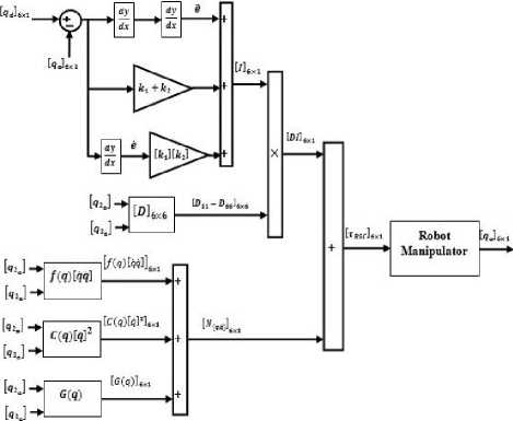
Fig. 1. Block diagram of robust backstepping controller

This computational burden has an effect on the performance of the control algorithm and imposes constraints on the hardware/software architecture of the control system. By only computing the dominant parts of the robot dynamics, this computational burden can be reduced. These drawbacks of the backstepping controller makes it necessary to consider control algorithms that compensate for both model uncertainties and for approximations made during the on-line computation of robot dynamics. The next section provides robust modifications of the backstepping controller described in this section. Fig. 1 shows the block diagram of backstepping controller.

Robust Backstepping Control: When there are uncertainties in the spherical motor dynamics due to modeling inaccuracy and computational relaxation, robust controllers are ideal for ensuring system stability. When the system dynamics are completely known, the required torque control vector for the control of the spherical motor is given by (12) and (13). In the presence of modeling uncertainties, a reasonable approximation of the torque control input vector is given by

• У = хld + ([Kp] + [Kd])(xld - Xi) +

([К р ]№-Х а

Td = [Я]у + C(15)

where [я] and C are estimates of the inertia and coriolis terms in the spherical motor dynamics; and у is given by (13). The uncertainty on the estimates are expressed as

[C] = [Я] - [Я]

• [C] = [C] — [C]

These uncertainties account for both imperfect modeling and intentional computational simplification. Application of the approximate control vector given by (14) leads to the following expression for the closed loop dynamics:

[Я]х2 + С = [Я]у + C

Since the inertia matrix [H] is symmetric and positive definite, the closed loop dynamics in (17) can be rewritten as

• *i = у - q

where q = ([/] - [Я]"^Я])у - [Я]"lC

Substitution of (13) for у in (18) results in the following expression for the closed loop error dynamics.

Xi + (И + [^])Я?1 + [Kp] [Kd]xi = q

Defining a new error state vector,

• *ll

xj f=[

the error dynamics in (20) can be expressed as f=[F]f+[D](x м-у + q )

Where [F] = [[®]   [^]] and [D] = [[^]] are block

[]  [][]

matrices of dimensions Д6Х6 and Д6ХЗ respectively. Since is a nonlinear function of the position and velocity state vectors, the system error dynamics in the above equation are nonlinear and coupled. The backstepping controller developed in the previous section cannot guarantee system stability. The Lyapunov direct method is, however, used to design an outer feedback loop on the error dynamics that compensates for the system uncertainty contributed by .

Supposed that is the universe of discourse and is the element of U, therefore, a crisp set can be defined as a set which consists of different elements ( ) will all or no membership in a set. A fuzzy set is a set that each element has a membership grade, therefore it can be written by the following definition;

A = {х,д_л(х)|х еХ};Ле{/ (24)

Where an element of universe of discourse is , is the membership function (MF) of fuzzy set. The membership function (ДлМ) of fuzzy set A must have a value between zero and one. If the membership function p_A (x) value equal to zero or one, this set change to a crisp set but if it has a value between zero and one, it is a fuzzy set. Defining membership function for fuzzy sets has divided into two main groups; namely; numerical and functional method, which in numerical method each number has different degrees of membership function and functional method used standard functions in fuzzy sets. The membership function which is often used in practical applications includes triangular form, trapezoidal form, bell-shaped form, and Gaussian form.

Linguistic variable can open a wide area to use of fuzzy logic theory in many applications (e.g., control and system identification). In a natural artificial language all numbers replaced by words or sentences.

If - then Rule statements are used to formulate the condition statements in fuzzy logic. A single fuzzy If - then rule can be written by

If x is A Then у is В (25)

where A and В are the Linguistic values that can be defined by fuzzy set, the - of the part of “x is A” is called the antecedent part and the then - par t of the part of “у is В” is called the Consequent or Conclusion part. The antecedent of a fuzzy if-then rule can have multiple parts, which the following rules shows the multiple antecedent rules:

if e is NВ and e is ML then T is LL (26) where e is error, e is change of error, NВ is Negative Big, ML is Medium Left, T is torque and LL is Large Left. If - then rules have three parts, namely, fuzzify inputs, apply fuzzy operator and apply implication method which in fuzzify inputs the fuzzy statements in the antecedent replaced by the degree of membership, apply fuzzy operator used when the antecedent has multiple parts and replaced by single number between 0 to 1, this part is a degree of support for the fuzzy rule, and apply implication method used in consequent of fuzzy rule to replaced by the degree of membership. The fuzzy inference engine offers a mechanism for transferring the rule base in fuzzy set which it is divided into two most important methods, namely, Mamdani method and Sugeno method. Mamdani method is one of the common fuzzy inference systems and he designed one of the first fuzzy controllers to control of system engine. Mamdani’s fuzzy inference system is divided into four major steps: fuzzification, rule evaluation, aggregation of the rule outputs and defuzzification. Michio Sugeno uses a singleton as a membership function of the rule consequent part. The following definition shows the Mamdani and Sugeno fuzzy rule base

Based on foundation of fuzzy logic methodology; fuzzy logic controller has played important rule to design nonlinear controller for nonlinear and uncertain systems [20-32]. However the application area for fuzzy control is really wide, the basic form for all command types of controllers consists of:

Mamdani F . R¹ :

у is В then z is C Sugeno   F . R¹ :

у is В then     f ( x , У ) is C

• •    Input fuzzification (binary-to-fuzzy[B/F]conversion)

• •    Fuzzy rule base (knowledge base)

• •    Inference engine

• •    Output defuzzification   (fuzzy-to-binary    [F/B]

conversion).

Fig 2 shows the block diagram of Fuzzy inference

When X and у have crisp values fuzzification calculates the membership degrees for antecedent part. Rule evaluation focuses on fuzzy operation ( AND / OR ) in the antecedent of the fuzzy rules. The aggregation is used to calculate the output fuzzy set and several methodologies can be used in fuzzy logic controller aggregation, namely, Max-Min aggregation, Sum-Min aggregation, Max-bounded product, Max-drastic product, Max-bounded sum, Max-algebraic sum and Min-max. Two most common methods that used in fuzzy logic controllers are Max-min aggregation and Sum-min aggregation. Max-min aggregation defined as below

Hu ⁽ x_k , Ук , и )= в ⋃ ^Ti=l^{FRi (} x_k , Ук , и ⁾

=      2 min'_i=l 0 hRpq ⁽ Xk , Ук ), Fp_m ⁽ и )13

The Sum-min aggregation defined as below

Bu ( x_k , Ук , и )= в ⋃ ^rt^l^FRt ( x_k , Ук , и ) =∑ min^T_l=1 0 ^^Rpq ( x_k , Ук ), B_Pm ( U )1

engine.

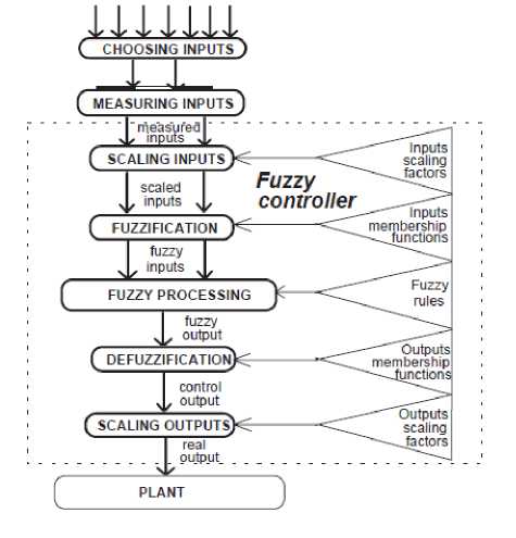
Fig. 2. Fuzzy Controller operation

where r is the number of fuzzy rules activated by x_k and Ук and also fl j i=l^FRl ( Xk , Ук , и ) is a fuzzy interpretation of i - t ℎ rule. Defuzzification is the last step in the fuzzy inference system which it is used to transform fuzzy set to crisp set. Consequently defuzzification’s input is the aggregate output and the defuzzification’s output is a crisp number. Centre of gravity method ( COG ) and Centre of area method ( COA ) are two most common defuzzification methods, which COG method used the following equation to calculate the defuzzification

The backstepping controller for continuum robot is calculated by;

U в . s ⁼      . + D . I

Where _. is backstepping output function, _. is backstepping nonlinear equivalent function which can be written as (49) and I is backstepping control law which calculated by (1)

. =[ f + C + G ^]

COG ( x_k , Ук )

^∑ jUj ^∑ ^=1 ․ Bu ( Xk , Ук , Ui ) ∑∑/=1․ Bu ( Xk , Ук , Ui )

We have

and COA method used the following equation to calculate the defuzzification

I =[ ̈+( Ki + K₂ )× e +( Ki × K₂ )∙ ̇]      (34)

Based on above formulation, FIS in this research has an input ( N ( q , ̇) and an output( U fuzzy ).

COA ( x_k , Ук )

^∑ НИ ․ Bu ( Xk , Ук , Ui ) ^∑ tBu .( x_k , Ук , Ui )

∑ i eT^(X)

Where COG ( x_k , Ук ) and COA ( x_k , Ук ) illustrates the crisp value of defuzzification output, U[ ∈ и is discrete element of an output of the fuzzy set, l^u .( Xk , У к , U[ ) is the fuzzy set membership function, and T is the number of fuzzy rules.

To estimate the nonlinear term of backstepping controller fuzzy inference system is used in serial with nonlinear dynamic part

^ ^=., = tV + C + G)l

♦Г-ч*      (36)

4—4=1

Based on above formulation the formulation of backstepping fuzzy control is;

Most robust control designs are based on the assumption that even though the uncertainty vector q is unknown, some information is available on its bound. In designing the robust backstepping controller, a robust term that compensates for the uncertainty in the system dynamics is added to the control law in (50) and (51).

Fuzzy backstepping controller is robust and stable but in presence of unlimited uncertainty gain tuning method based on fuzzy estimator is presented. In this method the fuzzy out port is used to estimate the system dynamic and also is use to gain tuning.

To reduce the error and increase the stability and robust adaptive methodology is used as a follows;

F ⁽q,q) = e ^1T £ ⁽ q,q)

= J# ¹ e ⁽q,q) ,...,6m e ⁽q,q) ]

The adaptation law is given by

¹ = -FijS j£⁽ q, q)              ⁽³⁹⁾

Where j = 1, ,„,m and r_Tj — Г₃j are positive diagonal matrices.

• IV.    Result and Discussion

To validate this research backstepping controller and proposed method is compared. These controllers are tested and implemented in MATLAB/SIMULINK.

Tracking performances: In proposed controller the gain is adjusted online depending on the last values of error ( e ) and change of error (e) by gain updating factor ( a ). Figure 3 shows tracking performance in proposed method, and backstepping controller without disturbance for step trajectory.

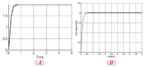
Fig. 3. Tracking performance a) proposed method b)Backstepping

Based on Figure 3 it is observed that, the overshoot in proposed method and backstepping controller are 0%, and rise time in proposed method is 0.48 seconds and in backstepping controller is about 0.6 seconds.

Disturbance rejection: Figure 4 shows the power disturbance elimination in proposed and BSC with disturbance for desired trajectory. In this part between t=0 and t=3 load moves to position 1. From t=2 sec to t=3 sec manipulator is carried load and expected to reach to position 2 at t=5 sec and disturbance is added to first link, Figure 5 is shown this situation.

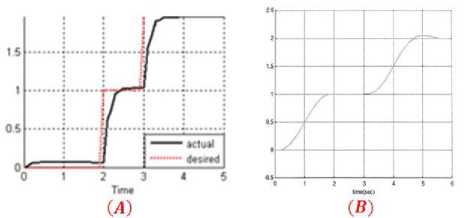
Fig. 4. Disturbance Rejection: a) proposed method b)Backstepping

The disturbance rejection is used to test the robustness comparisons of these two controllers for desired trajectory. Based on Figure 4; by comparing disturbance trajectory response in proposed method and and BSC, proposed method overshoot is about (0%) and BSC’s overshoot is about (0.4%). Proposed method’s rise time (0.48 seconds) is lower than BSC (0.53 second).

Fig. 5. Complicated situations applied into two controllers

• V.    Conclusion

According to this research, gain updating intelligent backstepping controller is introduced. This research has two objectives: design a Proportional-Derivative (PD) fuzzy system to compensate the system model uncertainties and design tuning gain adaptive methodology according to high quality partly nonlinear methodology. The fuzzy controller is used in this method to system compensation. In real time to increase the system robust fuzzy logic theory is applied to backstepping controller. To approximate a time-varying nonlinear dynamic system, a fuzzy system requires a large amount of fuzzy rule base. The adaptive laws in this algorithm are designed based on the Lyapunov stability theorem.

Acknowledgment

The authors would like to thank the anonymous reviewers for their careful reading of this paper and for their helpful comments. This work was supported by the SSP Institute of Advance Science and Technology Program of Iran under grant no. 2014-Persian Gulf-2A.

Ali Shahcheraghi is currently working as a primary researcher in the laboratory of Control and Robotic, Institute of Advance Science and Technology, IRAN SSP research and development Center. His current research interests are in the area of nonlinear control, artificial control system and robotics.