Intelligent Application for Predicting Diabetes Spread Risk in the World Based on Machine Learning

Published Online on June 8, 2025 by MECS Press

Information technologies today are the engine of development and evolution in many areas of human activity, from general-purpose systems to the sphere of critical technologies. The efficiency of the processes that they allow to automate depends on the quality and reliability of the use of software and hardware complexes. Systems of general-purpose information technologies include mass-operated systems, in particular, software systems that can be freely downloaded from marketplaces and installed locally on both mobile devices and users' computers. Critical systems include systems that have a direct impact on the life and health of people, the environment, etc. The implementation of information technologies in the field of medicine is especially relevant. They make it possible to analyse, monitor and predict the development of various diseases, improve the quality of life of patients, and also act as decision-making support systems for doctors when establishing a diagnosis. The current stage of human development is accompanied by the spread of diseases that tend to increase. Diabetes mellitus, cardiovascular diseases, strokes and heart attacks, Alzheimer's disease and multiple sclerosis, and cancers, which are mainly caused by genetics and lifestyle characteristics, geographical location of people, etc., are becoming widespread. Trends are observed regarding the increase in the number of patients to the scale of a pandemic analysing the spread of diabetes mellitus. Thus, according to forecasts of international organizations, there is a seven-fold increase in morbidity in 2045 compared to 2000, which is expressed in absolute terms as 700 million people compared to 145 million respectively. Given such disappointing indicators, the current task today is to build a comprehensive system for determining and predicting the development of diabetes mellitus.

Modern technologies and artificial intelligence (AI) are opening up new horizons in the field of medical research and the treatment of chronic diseases such as diabetes. Diabetes is a severe disease characterized by metabolic disorders and high blood glucose levels, which can lead to various complications, including heart, kidney, nervous system and vision damage. Therefore, timely detection and prediction of the development of this disease is crucial to prevent its complications. The development of artificial intelligence methods, in particular machine learning and deep learning, opens up prospects for creating practical tools for predicting the development of diabetes. These methods allow the analysis of large amounts of medical data, including laboratory tests, clinical indicators, lifestyle information and genetic factors, to identify individuals at high risk of developing diabetes at an early stage. Monitoring blood glucose levels is a defining part of life for people with diabetes, so it is essential, first of all, to ensure the convenience and accuracy of monitoring glucose levels, automated data transfer to a central repository, and prediction of its development.

Diabetes is generally categorized into three primary types: type 1, type 2, and gestational diabetes (which occurs during pregnancy). Type 1 diabetes is believed to result from an autoimmune response, where the body's immune system mistakenly attacks insulin-producing cells, leading to little or no insulin production. This type accounts for approximately 5–10% of all diabetes cases and typically appears rapidly, most often in children and young adults. Individuals with type 1 diabetes must take daily insulin to survive, and currently, there are no known prevention methods. Type 2 diabetes, the most common form – affecting 90–95% of people with diabetes – occurs when the body becomes resistant to insulin or fails to use it effectively. It develops gradually over time and is usually diagnosed in adults. Since early symptoms may be mild or absent, regular screening is essential, especially for those at risk. Type 2 diabetes can often be prevented or delayed by maintaining a healthy weight, following a balanced diet, and engaging in regular physical activity. Gestational diabetes develops during pregnancy in women who did not previously have diabetes. Although it typically resolves after childbirth, it increases the mother's long-term risk of developing type 2 diabetes.

Additionally, children born to mothers with gestational diabetes have a higher likelihood of obesity and diabetes later in life. Risk factors for type 1 diabetes are less well defined but include a family history of the disease and younger age at onset, typically during childhood, adolescence, or early adulthood. Type 2 diabetes risk factors include being overweight, aged 45 or older, having a family history of the condition, being physically inactive, having prediabetes, or having a history of gestational diabetes. Fortunately, type 2 diabetes can often be avoided or postponed through proven lifestyle adjustments.

Given the increasing prevalence and risks associated with all types of diabetes, there is a pressing need to develop a comprehensive system that combines both hardware and software solutions. Such a system should facilitate continuous data collection, management, and predictive analysis to monitor and support diabetes prevention and care.

The research purpose is to study the methods, software, and hardware used to process data in blood sugar monitoring systems. The object of the research is the processes of data collection and accumulation, as well as forecasting the development of diabetes mellitus. The subject of the study is the methods and means of data accumulation and forecasting the development of diabetes mellitus. The following tasks are set in the master's qualification work to achieve this goal:

• •    analyse scientific publications on factors influencing the development of diabetes mellitus;

• •    investigate existing software and hardware and other solutions for detecting and regulating the level of glucose

in human blood, accumulating and processing such data;

• •    propose an architecture and possible ways to implement a software and hardware system for collecting, accumulating and predicting blood glucose levels;

• •    create models and algorithms for predicting the development of diabetes mellitus based on existing open data;

• •    implement software to predict the development of diabetes mellitus.

When solving the tasks of the qualification work, the following methods and tools were used: analysis and generalization - when analysing statistical data on the incidence of diabetes mellitus and choosing ways to implement a blood sugar monitoring system; set theory and machine learning methods – when formalizing and building a conceptual model of the distributed architecture of the monitoring system and when predicting the development of diabetes mellitus; design and programming – when implementing a software model for predicting the development of diabetes mellitus; experiment and measurement – when assessing the accuracy of the prediction results and identifying factors with the most significant impact on the development of diabetes mellitus. This work focuses on the use of machine learning methods to predict the risk of developing type 2 diabetes mellitus based on the Pima Indians Diabetes dataset. The object of the work is the Pima Indians Diabetes dataset. The goal of the work is to develop and train a k-nearest neighbour (k-NN) model that is able to classify individuals accurately by the level of risk of developing diabetes. It is necessary to perform to achieve this goal:

• •    comprehensive data cleaning, including missing value filling and data normalization, to ensure the reliability of the results;

• •    optimize the model hyperparameters to find the best value for the number of neighbours for k-NN that maximizes the prediction accuracy;

• •    determine and analyse the leading performance indicators of the model, such as the error matrix, precision, completeness, F1 score, ROC-curve, and AUC score. It will allow us to evaluate the model’s ability to correctly classify cases with high and low risk of developing diabetes.

The scientific novelty of the obtained research results lies in the following:

• •    For the first time, algorithms for the functioning of a glucometer and a global information system for managing medical data were proposed, which together constitute a system for 24-hour monitoring and management of the patient's blood glucose level, which makes it possible to ensure the collection, processing and prediction of the appearance or development of diabetes mellitus.;

• •    For the first time, a conceptual model of a distributed architecture of a data collection and processing system for monitoring blood sugar levels has been constructed and mathematically presented, which includes a set of local and central control nodes and allows for the exchange of messages and the prediction of the development of the disease.

2.    Related Works 2.1.    Basic Principles of Diabetes

The implementation of the proposed solution for the use of software and hardware in the implementation of blood sugar monitoring systems allows for 24-hour monitoring and prediction of the potential occurrence and development of diabetes. The relevance of the work lies in the need to optimize medical care, improve the quality of life of patients, and reduce the economic burden associated with the treatment and complications of diabetes. The use of AI for diabetes prediction can significantly improve the processes of diagnosis, monitoring, and treatment, contributing to the transition from reactive treatment to a proactive and personalized approach in medicine. This work is aimed at studying data and developing an artificial intelligence model that will allow the prediction of the development of diabetes with high accuracy based on the analysis of various patient data. The results can be used to develop new clinical recommendations and strategies for managing the risk of developing diabetes.

Diabetes mellitus (DM) is one of the most commonly diagnosed diseases in the world. According to the International Diabetes Federation, more than 439 million people will be diagnosed with diabetes by 2030. Approximately 2–5 million patients die from DM each year. Diabetes mellitus is one of the most significant global health challenges. According to the World Health Organization, the number of people with diabetes has increased rapidly from 108 million in 1980 to more than 422 million in 2014 [1]. This number is projected to continue to increase, especially in developing countries.

Diabetes mellitus significantly increases the risk of developing serious complications, reduces quality of life and increases mortality. The main factors contributing to the increase in morbidity include an ageing population, increasing obesity, and lifestyle changes such as insufficient physical activity and an unbalanced diet [2]. An essential part of fighting the diabetes epidemic is raising awareness about the risk factors and the importance of early detection. Despite the high prevalence of the disease, no practical method has yet been proposed to reduce its incidence, although various methods are currently used to treat and control the disease. Almost all the foods we eat are broken down into sugar (called glucose) and released into the bloodstream. When blood glucose levels rise, this signals the pancreas to secrete insulin. It acts as a key for the sugar in the blood to enter the cells of your body to be used as energy. If you have diabetes, it means that your body does not produce enough insulin or does not use it properly. When there is not enough insulin or the cells stop responding to insulin, too much blood sugar remains in the blood. People with diabetes are at high risk of developing diseases such as heart disease, kidney disease, stroke, eye problems, nerve damage, and more. It is reportedly the fourth leading cause of death in most human societies.

Diabetes mellitus is divided into three main types: type 1 diabetes, type 2 diabetes, and gestational diabetes [3]. Type 1 diabetes occurs when the body’s immune system destroys the insulin-producing cells in the pancreas. This type of diabetes is most commonly diagnosed in children and young adults but can develop at any age. Type 2 diabetes, which accounts for approximately 90–95% of all cases, usually develops in adults and is associated with insulin resistance and insufficient insulin production. Gestational diabetes can occur in women during pregnancy and usually resolves after delivery, but increases the risk of developing type 2 diabetes later in life. These types of diabetes have different causes and treatments, emphasizing the need for accurate diagnosis and an individualized approach to each patient.

Type 2 diabetes is the most common type of diabetes. It has multiple risk factors that can influence its development. Genetics plays a significant role. However, genetic factors interact with a number of environmental factors, including lifestyle. Physical inactivity and being overweight significantly increase the risk of developing the disease. Other factors include age and ethnicity. Diet is also an essential factor: high-calorie foods rich in simple carbohydrates and saturated fats can contribute to insulin resistance [4]. Understanding these factors allows us to more effectively identify individuals at high risk of developing diabetes and to take preventive measures:

• •    Genetics, such as having a first-degree relative with diabetes, significantly increases the risk of developing the disease. Heredity plays a key role in the predisposition to type 1 and type 2 diabetes. Genetic mutations can affect the body's ability to produce or use insulin;

• •    Lifestyles, such as physical inactivity and unhealthy eating habits, are important risk factors. Regular exercise and a healthy diet can significantly reduce the risk of developing type 2 diabetes. On the other hand, high levels of sugar and fat intake increase the likelihood of developing diabetes and its subsequent complications;

• •    Obesity, as excess weight, especially abdominal fat, causes insulin resistance, which is a significant factor in the development of type 2 diabetes. Weight management can significantly reduce the risk of developing diabetes;

• •    Age, in particular, the risk of developing diabetes increases with age, especially after the age of 45. It is due to decreased physical activity, decreased muscle mass, and changes in metabolic patterns;

• •    Ethnicity, for example, some ethnic groups, such as African Americans, Hispanics, and South Asians, are at higher risk of developing diabetes. It may be due to genetic factors, as well as cultural factors and access to healthcare.

If you have any of the following symptoms of diabetes, see your doctor about testing your blood sugar: passing a lot of urine, often at night; feeling very thirsty; losing weight without trying; feeling very hungry all the time; having blurred vision; having numbness or tingling in your hands or feet; feeling very tired; having dehydrated skin; having sores that heal slowly; – having more infections than usual. There is no cure for diabetes yet, but losing weight, eating a healthy diet, being active, and getting your diabetes diagnosed early can really help. Diabetes can lead to many serious complications that not only affect the quality of life of patients but can also be life-threatening. The importance of early detection is to prevent or minimize these complications:

• •    Cardiovascular diseases, in particular diabetes, significantly increase the risk of developing cardiovascular diseases, such as coronary artery disease, myocardial infarction, and stroke. High blood glucose levels can damage the inner lining of blood vessels, contributing to atherosclerosis. These conditions complicate blood circulation and can ultimately lead to serious cardiac events that require immediate medical attention;

• •    Diabetic neuropathy is damage to nerve fibres throughout the body, which most often affects the lower extremities. Symptoms include pain, tingling, and loss of sensation, which significantly reduces quality of life and increases the risk of injury due to loss of sensation. In severe cases, neuropathy can lead to foot deformity, requiring orthopaedic intervention;

• •    Diabetic retinopathy is one of the leading causes of vision loss among people of working age. High blood sugar levels damage the small blood vessels in the retina, which can lead to bleeding, scarring, and, ultimately, retinal detachment. Regular eye exams and timely treatment with laser or other methods can help prevent vision loss;

• •    Kidney failure, particularly diabetes, is one of the leading causes of chronic kidney failure. High glucose levels gradually damage the kidneys, particularly the filtering structures, which can eventually lead to the need for dialysis. Early detection of changes in kidney function and aggressive management of blood sugar and blood

pressure can prevent or delay progression to end-stage kidney disease;

• •    Diabetic foot is a serious complication that involves nerve damage and poor circulation in the feet, which can lead to infections, ulcers, and even amputations. Diabetic patients should regularly check their feet for injuries, cracks, or ulcers and use special footwear to prevent injuries. Early treatment of infections and timely surgical intervention for ulcers can prevent more serious consequences.

• 2.2.    The Role of Artificial Intelligence in Medicine

  AI in medicine has deep roots, dating back to the mid-20th century when the concepts and algorithms that gave rise to this field were first developed. Early research focused on creating systems that could mimic the clinical thinking of doctors. One of the first known systems was the MYCIN program [6], developed in the 1970s at Stanford University. MYCIN used rules to diagnose infectious diseases and recommend antibiotic treatment, although it was never used in clinical practice due to the limitations of the technology at the time. With the advent of more powerful computers and the development of machine learning, AI began to be integrated into medicine with new force. In the 1980s and 1990s, numerous diagnostic and navigation systems were created based on artificial intelligence, helping medical professionals make decisions based on large amounts of data. These systems used knowledge bases filled with data about symptoms, treatments, and patient feedback [7]. The current stage of AI in medicine is characterized by the use of sophisticated deeplearning algorithms that can analyse medical images, interpret medical records, and even predict potential medical conditions based on genetic information. For example, deep learning systems such as those developed by Google Health and DeepMind have demonstrated the ability to detect diabetic retinopathy and other eye diseases at the same or even better than trained professionals [7]. The value of AI in medicine continues to grow due to its ability to process and analyse large amounts of data faster and more accurately than humans can. It not only increases the efficiency of medical research and diagnostic procedures but also contributes to the development of personalized approaches to treatment, opening up new opportunities for the prevention and treatment of diseases at the individual level.

Regular monitoring of blood glucose levels, adherence to diet, physical activity and proper medication are key aspects of treatment. In addition, regular consultations with doctors and other health professionals allow you to detect any changes in your health in time and adjust therapy. It is also essential to pay attention to your psycho-emotional state, as stress and depression can negatively affect the course of the disease.

Adequate control of diabetes requires an integrated approach that includes medication, lifestyle changes, regular self-monitoring, and patient education. Medication is the mainstay of treatment for type 1 diabetes, where patients require insulin because their bodies cannot produce it. Insulin is administered by injection or with insulin pumps, allowing for precise control of blood sugar levels. For type 2 diabetes, different classes of blood glucose-lowering drugs are used, such as metformin, sulfonylureas, insulin, and others [5]. It is crucial to tailor treatment to each patient, taking into account their overall health, age, lifestyle, and other medical conditions. Lifestyle changes include recommendations for a healthy diet and physical activity. A healthy diet for people with diabetes includes limiting simple carbohydrates, increasing fibre, and balancing protein and fat intake. Physical exercise helps maintain a healthy weight, improve insulin resistance, and improve overall health. At least 150 minutes of moderate aerobic exercise per week is recommended. Patients with diabetes should regularly monitor their blood glucose levels using glucometers. It allows patients to track the effects of diet, physical activity, medications, and stress on glucose levels.

Regular self-monitoring is critical to avoiding hypo- and hyperglycaemic states, which can be dangerous [5]. It is also essential that patients are well-educated about all aspects of their condition, including how to manage their diabetes, how to recognize and treat hypo- and hyperglycaemia, and how to prevent complications. Effective diabetes education programs can include individualized education, group classes, and seminars, as well as educational materials and online resources. Psychological support is an important aspect. A diagnosis of diabetes can cause emotional distress. Mental health support is an essential component of comprehensive care for people with diabetes. It may include access to psychological counselling, support groups, and other resources to help manage stress and emotions.

AI is revolutionizing medicine, particularly through the introduction of advanced technologies and tools that improve the diagnosis, treatment, and monitoring of diseases. The application of AI in medicine encompasses a wide range of technologies, each with its characteristics and areas of application. Machine learning is one of the main components of AI in medicine. It includes algorithms that can learn from experience without being explicitly programmed for each task. In medicine, machine learning is used to analyse large amounts of data, from laboratory test results to medical records. These algorithms are able to identify patterns and abnormalities that may not be obvious to the human eye. Deep learning, a subcategory of machine learning, involves models that mimic the structure and functioning of the human brain using artificial neural networks. It is beneficial for processing and analysing medical images, such as X-rays, MRIs, or ultrasounds. Deep learning can detect subtle pathological changes in images that may indicate early stages of diseases such as cancer or heart disease. Natural language processing (NLP) is used to analyse medical records, transforming unstructured medical information into a structured form that can be easily interpreted and used to support clinical decisions. NLP can help identify trends in symptoms, treatments, and outcomes and standardize records for further analysis. Computer vision is another crucial AI tool used to identify, classify, and quantify images. In medicine, it can be used to automatically detect abnormalities in medical images, enabling faster and more accurate diagnoses. Robotic surgery, while not a purely software aspect of AI, uses machine learning algorithms to control surgical instruments, allowing for more precise surgeries with smaller incisions. It helps patients recover faster and reduces complications.

Overall, these technologies and tools are creating the basis for new approaches in medicine, increasing the efficiency of diagnostics and treatment, and providing more personalized healthcare. Artificial intelligence has the potential to radically change medical practice, making it more accurate, efficient and accessible. Disease prediction and diagnosis using AI opens up new possibilities for medical science. AI can significantly improve the accuracy of diagnostic procedures and the ability to predict the future development of patient health based on the analysis of vast data [8]:

• •    diagnostic accuracy, for example, AI uses machine learning algorithms to analyse medical images such as X-rays, MRIs, and ultrasound scans. Deep learning systems, especially convolutional neural networks, are effective at recognizing pathological changes in medical images that are often missed by the human eye. AI algorithms can detect minimal deviations from the norm, which allows for the diagnosis of diseases at an early stage;

• •    disease risk prediction, for example, artificial intelligence models use a patient’s medical history, genetic information, and lifestyle habits to predict the likelihood of developing diseases such as diabetes, heart disease, and cancer. The use of biomarkers, such as biochemical indicators in the blood, contributes to the accurate determination of risk. Predictive models allow the identification of individuals at high risk of developing a disease before symptoms appear, which can increase the effectiveness of preventive measures;

• •    early detection and intervention, for example, through the analysis of medical data, AI allows the detection of minimal changes in health that may indicate the onset of a disease. Early intervention based on AI data can include recommendations for changes in diet, exercise, or medication. Predicting serious complications in chronic patients (for example, predicting hypoglycaemic states in patients with diabetes) can help avoid lifethreatening situations;

• •    Optimization of health care, in particular, AI contributes to a more efficient allocation of medical resources, such as determining the need for specialized examinations or interventions. Automation of routine diagnostic procedures reduces the burden on medical staff and shortens waiting times for patients. With the help of AI, it is possible to analyse the effectiveness of different treatment methods and choose the most effective ones based on large volumes of clinical data.

It opens up new possibilities for medicine, making the processes of prediction and diagnosis not only faster but also more accurate, leading to improved overall quality of healthcare, reduced costs, and better outcomes for patients. Personalized medicine, often referred to as data-driven medicine or precision medicine, is seen as the future of healthcare. This approach uses detailed analysis of each person’s genetic information, biomarkers, and other characteristics to develop individualized treatment and prevention plans [9]. Here are some more details about the prospects and future of personalized medicine:

• •    ndividualized treatment plans, in particular, the use of artificial intelligence in personalized medicine, allows doctors to better understand how different factors, such as a patient’s genetic profile, can affect a disease and its treatment. It leads to the development of more effective treatment plans that can reduce the risk of side effects and improve treatment outcomes;

• •    Genomics and pharmacogenetics, for example, AI helps analyse vast amounts of genomic data to identify mutations that affect the risk of developing diseases. Such analysis can also indicate how a patient will respond to certain drugs, thereby allowing for the selection of the most effective drugs without unnecessary trial and error;

• •    Predicting treatment responses based on the use of machine learning to predict treatment responses, which changes approaches to patient management. AI models can predict how likely patients are to respond to treatment with certain drugs, allowing for individual sensitivity to drugs or the likelihood of resistance;

• •    Bioinformatics and data integration, in particular, personalized medicine, requires the integration of diverse data, including genetic, biomedical, epidemiological and clinical data. Bioinformatics plays a key role in combining these data into holistic models that allow for deeper analysis of the relationships between different types of information and increase the accuracy of medical predictions;

• •    Ethical and legal challenges based on the implementation of personalized medicine also face ethical and legal challenges, in particular, issues of confidentiality and access to genetic information. It requires the development of new regulatory frameworks that would protect patients' rights and, at the same time, promote scientific research;

• •    The future and innovation, in particular, the prospects for personalized medicine look promising given the rapid development of biotechnology and artificial intelligence. In the future, it is possible to create even more accurate tools for monitoring and treating diseases at the individual level, which will change medical practice;

• •    Interaction with patients and healthcare professionals, such as the increasing adoption of personalized medicine, requires a new level of interaction between patients and doctors. Healthcare professionals need new skills to interpret complex data and to communicate with patients about their health based on genetic information and individual risks.

• 2.3.    Artificial Intelligence and Diabetes

These aspects demonstrate that personalized medicine has the potential to radically change medical practice, making treatment more targeted and effective while creating new challenges and opportunities for medical science and practice.

Using AI to identify diabetes risk could revolutionize prevention and early diagnosis. It is possible thanks to advanced machine learning algorithms that analyse large datasets and identify potential risks before symptoms appear [9]. AI algorithms are used to analyse genetic data to identify markers associated with an increased risk of diabetes. These genetic markers can include mutations or gene variants that have been linked to diabetes in scientific studies. Risk factor screening: Algorithms can analyse a wide range of risk factors, such as age, weight, family history, physical activity levels, eating habits, and pre-existing medical conditions such as hypertension or metabolic disorders. Previous medical outcomes: Using AI to analyse a patient’s historical medical data, including blood glucose and haemoglobin A1c test results, which may indicate an earlier risk of developing diabetes. Lifestyle analysis: AI can process lifestyle data collected through mobile apps and other sources to determine how daily habits may affect the risk of developing diabetes. For example, low physical activity and a high-calorie diet are known risk factors. Risk modelling – modern AI technologies can model different scenarios based on the data provided to help predict future health outcomes based on current trends and changes in patient behaviour. The availability of AI tools in medicine, particularly in the diagnosis and treatment of diabetes, is a critical issue affecting global health. Despite the significant potential of AI to improve outcomes and reduce costs, there are a number of challenges that limit the widespread adoption of these technologies in clinical practice, especially in resource-limited settings [10]:

• •    the cost of technology, in particular, one of the main barriers is the high cost of developing and implementing AI systems. Developing practical algorithms requires significant investments that not all healthcare institutions can afford;

• •    the need for skilled professionals, in particular, the use and management of AI requires the availability of skilled professionals such as data engineers, analysts and health informatics, which are often in short supply, especially in developing countries;

• •    data infrastructure, for example, the effective use of AI requires a reliable IT infrastructure to collect, store and process large amounts of data. In many regions, the necessary IT infrastructure is lacking, which limits the possibilities of using advanced analytical tools;

• •    legal and ethical issues, in particular, the legislation governing the use of medical data and AI varies between countries, which can complicate international cooperation and technology exchange. In addition, there are issues of confidentiality and data misuse;

• •    Educational barriers, such as healthcare professionals needing additional education and training to effectively use AI. The need for continuous education and retraining can be burdensome and require time and resources;

• •    implementation in clinical practice, in particular, the integration of AI into clinical practice requires clear evidence of effectiveness and safety. Clinical trials to validate AI tools can be lengthy and expensive;

• •    acceptance of technologies, as there is scepticism from both patients and healthcare professionals about the use of AI, which can affect the acceptance and implementation of new technologies. Fears about the loss of personal contact between doctor and patient may also play a role;

• •    adaptation of technologies, i.e. the need to adapt existing AI systems to local conditions and needs, can be complex. Cultural, linguistic and demographic differences require individualized approaches;

• •    technical limitations, for example, AI tools may have limitations due to insufficient accuracy, problems with data collection, or insufficient ability for general adaptation.

Overcoming these challenges requires a concerted effort by governments, education, healthcare and the technology industry to create accessible, effective and safe AI tools that can improve the treatment and diagnosis of diabetes globally. Data collection and analysis are critical steps in the process of using AI to predict the development of diabetes. It is a process that requires high precision and care because the effectiveness of further analysis and the accuracy of predictions depends on the quality of the data collected [10, 11]. In the beginning, it is necessary to determine which data sources will be most relevant for the study. These can be medical records, laboratory test results, patient lifestyle data, as well as information from wearable devices that monitor health:

• •    data collection after data sources have been identified should be systematic and standardized to ensure consistency and reproducibility of results;

• •    data quality verification, in particular, is critical to ensure that the data used is accurate, complete, and up-to-date. Incomplete or inaccurate data can lead to errors in prediction and analysis;

• •    Data normalization, as different sources may provide data in different formats, is necessary for their integration. It includes unifying measurement scales, converting data to a standard format, and resolving data incompatibility issues;

• •    handling missing values, as missing data is a common problem in health data. It is vital to identify techniques for handling these gaps, such as imputation based on existing data;

• •    identifying and handling outliers that may distort the results of analysis and prediction. It is essential to identify and adequately handle outliers so that they do not affect the overall conclusions;

• •    modelling based on the use of machine learning algorithms to develop predictive models. This process includes training, testing, and validating models on collected data;

• •    evaluating the model using metrics such as accuracy, sensitivity, specificity, and area under the ROC curve;

• •    iterating and optimizing to fine-tune parameters and select the best algorithms for specific data.

3.    Material and Methods 3.1.    Analysis of Statistics and Factors Influencing the Development of Diabetes Mellitus

Integrating AI into healthcare is a complex process that requires careful consideration of regulatory, technical, educational, and ethical aspects. Regulatory regulation plays a critical role in ensuring the safety and effectiveness of AI-based medical products. It includes certifying new technologies to ensure that they meet quality and safety standards. It is also necessary to ensure that AI-based systems meet all privacy and data confidentiality requirements established in the healthcare industry [12]. Technical integration requires compatibility of AI with existing IT systems in hospitals, which can be a challenge due to the heterogeneity and obsolescence of some systems. It includes integration with electronic medical records, laboratory systems, and portable medical devices. It is also essential to ensure a high level of data protection to prevent unauthorized access and other data integrity risks. Professional training of healthcare professionals is a necessity for practical work with new technologies. Doctors and nurses need to be provided with appropriate training to ensure they understand the capabilities of AI, as well as the skills to interpret and use the results that these systems offer. Healthcare professionals must be able to integrate this data into the clinical context and make informed decisions based on it [12]. In addition to the technical and educational aspects, it is also essential to consider the ethical aspects associated with the use of AI in clinical practice. These include issues of confidentiality, informed consent of patients, and the potential impact of algorithmic errors on the health and well-being of patients. Taking these aspects into account is key to building trust and acceptance of AI in medicine.

Healthcare is always a big issue for any nation, and it is always a challenging task. The best indicator of the health of a country is the condition of the residents living there. Improving the healthcare system can directly lead to economic growth as a healthy person can prove to be a great asset to the nation and can effectively function in the workforce compared to an unhealthy person. Healthcare is the unification and integration of all the measures that can be taken to improve the healthcare system. Healthcare is about prevention, diagnosis and treatment. Improving healthcare should be a top priority. Using technology to improve healthcare has proven to be very beneficial. In hospitals today, diagnosing diabetes involves conducting a range of medical tests to gather essential information, which then guides the selection of appropriate treatment. Big Data Analytics has become increasingly important in the healthcare sector, where vast amounts of patient data are generated and stored. By applying big data techniques, healthcare professionals can analyze extensive datasets to uncover valuable insights, detect hidden patterns, and extract meaningful knowledge that supports accurate predictions and informed decision-making. Machine learning, in particular, offers powerful tools for the prevention, early detection, and treatment of a wide range of diseases.

Machine learning and data processing technologies are the best sources for improving the healthcare system. Manual detection or diagnosis done by doctors is time-consuming and inaccurate. Machines that are built to learn to detect diseases through machine learning and data mining can diagnose the problem better, and that too with high accuracy. Machine learning can not only prove helpful in analysing and predicting the disease. Still, it can also be useful in personalized treatment and behaviour modification, drug development and discovery of new patterns leading to new drugs and treatments, and clinical trial research. With the help of machine learning, we can do all these in a better way. Machine learning is considered one of the most critical functions of artificial intelligence that supports the development of computer systems that can learn from past experiences without the need to be programmed for each case. Machine learning is considered to be a pressing need in today’s situation, with the aim of eliminating human efforts by supporting automation with minimal flaws. The existing method of detecting diabetes is the use of laboratory tests such as fasting blood glucose and oral glucose tolerance. However, this method is laborious. We live in an era where data is generated exponentially, leading to the accumulation of huge data. Especially in the healthcare industry, the availability of data is large, but the need to extract knowledge from it is also significant; otherwise, the collection of big healthcare data will be useless if it is not used. Data mining and machine learning help to find helpful information that can be further widely used. In the healthcare industry, data mining and machine learning can be used to improve patient care, best practices, effective patient treatment, fraud detection, and more accessible healthcare services. Data mining can also be used to detect a plague outbreak earlier (prediction) by observing the trends in the symptoms/complaints of patients. Different prediction models have been developed and implemented by other researchers using variants of data mining methods, machine learning algorithms or also a combination of these methods [13]. In a study [14], a system using Hadoop and Map Reduce methods was implemented to analyse diabetic data. This system predicts the type of diabetes as well as the associated risks. The system is Hadoop-based and is cost-effective for any healthcare organization. In a study [15], the author used a classification technique to learn hidden patterns in a diabetes dataset. This model used naive Bayes and decision trees. The performance of both algorithms was compared, and their effectiveness was demonstrated.

In a study [16], a classification technique was used. The authors used the C4.5 decision tree algorithm to find hidden patterns from the dataset for efficient classification. In the study [17], an artificial neural network (ANN) was used in combination with fuzzy logic to predict diabetes. In [18], a hybrid prediction model was proposed, which includes a simple K-means clustering algorithm followed by a classification algorithm based on the result obtained from the clustering algorithm. The C4.5 decision tree algorithm is used to build the classifiers. In [19], a model using the Random Forest Classifier was proposed to predict the behaviour of diabetes. In [20], the C4.5 decision tree algorithm, neural network, K-means clustering algorithm, and visualization were used to indicate diabetes.

We propose to consider predicting the probability of diagnosing diabetes in the early stages using an ensemble machine learning method – XGBoost implemented in the Python programming language.

Diabetes mellitus is a chronic metabolic disease characterized by elevated blood glucose levels due to absolute or relative insulin deficiency [21]. According to the International Diabetes Federation, as of 2022, 537 million adults aged 20–79 years are currently living with diabetes worldwide. It is expected that by 2030, their number will increase to 643 million [22]. The global nature of the problem of increased incidence of diabetes mellitus has formed a complex medical and social situation, which is acquiring the characteristics and nature of a pandemic. Given the global trend towards the detection and spread of diabetes mellitus, this trend is also observed in Ukraine. In particular, over the past decade and a half, we have observed an increase in the prevalence of this disease by more than fifty per cent, and the number of cases has increased by more than 80%. Diabetes treatment aims to help people with this disease achieve near-normal glycemic levels to reduce the risk of long-term (e.g. vascular) complications while avoiding acute metabolic risks and maintaining the best quality of life. There are different types and stages of the disease. For example, type 1 diabetes is caused by an autoimmune reaction in which the human body damages the cells that are responsible for insulin. It affects its insufficiency and disruption of the body's functions. The probable cause of the development of diabetes is a specific structure at the gene level. At the same time, environmental factors, viral infections and immune system disorders are triggers that stimulate the development of diabetes [23]. A key factor in achieving reasonable glycemic control is self-management of the condition. Individuals with diabetes should [24-27]:

• •    control carbohydrate intake through food choices, an adaptation of eating behaviour to glycemic load;

• •    adhere to the principles of healthy eating;

• •    manage blood glucose levels using glucose-lowering drugs;

• •    monitor sugar levels using traditional blood tests or computer systems with appropriate sensors;

• •    provide physical activity to optimize glycemia and control body weight;

• •    organize activities in accordance with current glycemia levels and treatment requirements recommended by doctors.

• 3.2.    Analysis of Existing Types of Devices for Measuring Blood Sugar Levels

If rapid-acting insulin is used (to cover elevated glucose levels after meals), assessing carbohydrate load, adjusting insulin dose, and correcting elevated glucose levels are additional necessary practices of daily diabetes self-monitoring.

Ongoing or repeated episodes of high blood glucose (hyperglycemia) significantly increase the likelihood of developing serious long-term complications related to diabetes, such as diabetic retinopathy, neuropathy, and nephropathy, often accompanied by diabetic foot syndrome. Poor glycemic control is also linked to a heightened risk of acute metabolic events, including severe hypoglycemia and extreme hyperglycemia, which may lead to conditions like ketoacidosis or hyperosmolar coma [27–28]. Therefore, consistently engaging in effective self-management behaviours aimed at achieving stable blood glucose levels is essential for preserving health and minimizing the risk of complications and disease progression [29–30]. Nevertheless, research indicates that many individuals with diabetes have room for improvement in their self-care practices. It is especially relevant for patients who also experience mental health challenges, such as depression or diabetes-related emotional distress, which can further hinder effective self-management [31]. Given that self-care plays a central role in influencing diabetes outcomes, monitoring individual behaviours to identify gaps and offering targeted support may be a valuable addition to everyday clinical care. Evaluating self-management in individuals with diabetes is especially important when glycemic control remains consistently poor, as it helps to identify underlying issues and potential risks. Such assessments may also be necessary in research settings to explore factors that support improved diabetes care – such as psychosocial influences [32] – or to measure the effectiveness of specific interventions, such as diabetes self-management education programs. A key element in supporting self-management is the use of accessible and reliable tools for monitoring blood glucose levels. A systematic review of existing instruments for assessing diabetes self-care revealed a wide variety of tools developed for this purpose. However, many of these tools have been applied in only a small number of studies, and their psychometric properties have not been thoroughly tested. As a result, only a few available scales meet the rigorous standards recommended by experts. These issues limit the applicability of existing measurement tools. In 2013, the Diabetes Self-Management Questionnaire was introduced to provide a multifactorial assessment of diabetes behaviour, which plays a vital role in glycemic monitoring in the significant types of diabetes.

In direct comparisons, the DSMQ explained significantly more variation in glycemic control than the established standard self-management scale [33]. It has since been translated into multiple languages and used in many studies, confirming its potential value for research and practice. A recent systematic review identified the DSMQ as one of three diabetes self-management scales that meet the COSMIN guidelines for instruments that can be recommended for use and that produce results that are reliable [34-35]. However, technological innovations such as continuous glucose monitoring and automated insulin delivery have changed the timing and pathways of diabetes care [36-44]. In addition, an instrument that meets the requirements set by the organization [27] should better capture some specific aspects of self-management.

According to [32], in Ukraine, there is currently no possibility of building a comprehensive system for analysing and forecasting the trend of diabetes incidence since there are no organizational mechanisms and technical means for forming and processing statistics on the development of diabetes and mortality from this disease.

Regularly checking your blood glucose (sugar) levels is the only reliable method to determine whether your levels are within a healthy range. Most people cannot accurately sense their blood sugar levels based on physical symptoms alone, so proper testing is essential. It is achieved through various specialized devices.

• •    A compact device Glucometer that requires a small drop of blood, typically taken from the fingertip and placed on a test strip. The device then calculates the glucose concentration in the blood.

• •    The Flash Glucose Monitoring (FGM) method utilizes a sensor worn on the back of the upper arm. It continuously collects glucose data and transmits it to a dedicated reader or smartphone app, eliminating the need for finger pricks. It provides 24/7 monitoring, helping users track trends throughout the day and night.

• •    A continuous Glucose Monitoring (CGM) sensor is inserted under the skin to measure glucose levels continuously. CGM is particularly beneficial for individuals with unstable blood sugar control. The average annual cost, including sensors and maintenance, is approximately $5,000. For example, in Australia, the National Diabetes Services Scheme (NDSS) subsidizes CGM and FGM devices, as well as related diabetes care supplies like syringes, test strips, and insulin pump components.

• •    Ketone Testing is primarily recommended for individuals on insulin therapy. Ketone testing helps detect the presence of ketones, which can indicate severe metabolic conditions:

o Urine ketone strips change colour based on the ketone concentration in the urine.

o Blood ketone meters function similarly to glucometers, offering more precise measurements.

Glucose meters may malfunction or produce inaccurate results due to Device ageing, Exposure to moisture, heat, or dirt, Low or depleted batteries, Expired test strips, Incorrect meter calibration codes, Incompatible or improperly inserted test strips, Insufficient blood samples, Contaminants like sugar on fingertips before testing. To ensure reliable results, always follow the manufacturer’s instructions. Hands should be washed thoroughly with soap and water and then dried before testing to prevent contamination. Additional Considerations:

• •    CGM sensors must be replaced weekly and inserted in a new location on the body. Periodic cross-checks with traditional fingerstick methods are recommended to verify CGM accuracy.

• •    Flash glucose monitors should only be applied to clean, dry skin to ensure proper adhesion and performance.

• •    Replacement batteries for diabetes-related devices are typically available at electronics stores, but users should always confirm the correct battery type and installation method.

• 3.3.    Program Operation Algorithm

Diabetes can be diagnosed if the fasting blood glucose level is 126 mg/dL or higher. A typical fasting glucose test result is below 100 mg/dL. One of the main goals of diabetes treatment is to maintain blood glucose levels within a given target range. More than 400 million people worldwide live with diabetes, and they still suffer from the inconvenience of pricking their fingers several times a day to check their blood glucose levels. Various methods alternative to the finger prick method have been widely studied for determining blood glucose levels, including enzymatic or optical glucose sensors. However, they still have problems in terms of durability, portability, and accuracy. In a study [34], the research team introduced semi-continuous and continuous blood sugar monitoring with low maintenance costs without the pain of blood sampling, allowing patients to maintain quality of life through proper diabetes treatment and control. It is expected that the use of CGMS will increase, which currently stands at only 5%. The research team also conducted both an intravenous glucose tolerance test (IVGTT) and an oral glucose tolerance test (OGTT) with the sensor implanted in pigs in a controlled environment. According to the research team [34], the results of the initial in vivo proof-of-concept experiment showed a promising correlation between blood sugar levels and the frequency response of the sensor. The sensor demonstrates the ability to track blood sugar trends, and for actual implantation of the sensor, biocompatible packaging and foreign body reactions for long-term use need to be considered. In addition, an improved sensor interface system is under development. It should be noted that devices designed for continuous monitoring of blood sugar levels are currently practically not used in Ukraine, and only 5% of this type of equipment is used in the world. This is due to their cost and convenience for the patient. However, two types of glucometers are prevalent: invasive and non-invasive.

A characteristic feature of non-invasive glucose measurement devices is that they do not damage the skin, and measurements can be performed more often than with traditional glucometers. However, the disadvantage of such devices is that the accuracy of their measurement can cause significant errors in the event of impaired blood supply, the presence of coarse skin or calluses, and the monitoring itself, which must be carried out up to seven times a day. The essence of the functioning of non-invasive glucose meters is the analysis of the state of blood vessels. That is, indirect measurements are not provided. In addition, several functional models calculate glucose concentration in the blood based on the analysis of the state of the skin. It is enough to ensure the device's contact with a part of the human body to do this. Optical methods use different properties of light to interact with glucose depending on its concentration. The transdermal method involves measuring glucose levels through the skin using electrical pulses or ultrasound. Finally, thermal methods aim to measure glucose levels by detecting physiological parameters related to metabolic heat generation. Transdermal methods are affected by environmental changes, such as temperature and sweat [33], while the main limitation of optical technologies is that they depend on the properties of the matter being tested, such as skin colour [34]. MIR light only extends a few micrometres and can be used to analyse a blood sample.

On the other hand, NIR light penetrates the biological environment deeper, up to several millimetres. NIR has the potential to be used for non-invasive or minimally invasive blood analysis, even if the glucose absorption is not as high as in the MIR region. The most common non-invasive methods are listed below. When using near-infrared spectroscopy, glucose gives one of the weakest absorption signals in this infrared range per unit concentration of the main component in the body. Measuring glucose levels using near-infrared spectroscopy allows for the investigation of tissue depths in the range of 1 to 100 millimetres, with a general decrease in penetration depth with increasing wavelength. Near-infrared radiation penetrates the earlobe, the web, and the cuticle of the fingers or is reflected from the skin.

Another technology for noninvasive blood glucose monitoring is a spectroscope, which measures the absorption of far-infrared (FIR) radiation. It is part of the natural thermal spectrum and, with the appropriate device, allows the measurement of FIR absorption, which is present in natural thermal radiation or body heat. FIR spectroscopy is the only type of radiation technology that does not require an external power source. Raman spectroscopy measures scattered light, which is affected by the oscillations and rotations of the scattered light. Various Raman methods have been tested for blood, water, serum, and plasma solutions. Analytical problems include instability of the laser wavelength and intensity, errors due to other chemicals in the tissue sample, and long spectral acquisition times. [23] Photoacoustic spectroscopy uses an optical beam to rapidly heat the sample and create an acoustic pressure wave that can be measured with a microphone. The methods are also subject to the chemical effects of biological molecules, as well as the physical effects of changes in temperature and pressure. Glucose in the blood is responsible for providing the body with energy. For spectrophotometric experiments, Lambert's law of absorption notation is used and developed to express the absorption of light as a function of the concentration of glucose in the blood.

An algorithm is a set of instructions designed to perform a specific task. Therefore, the algorithm of the program operation is drawn up in the notation of an activity diagram (Fig. 1-2). According to this method, in order to conduct a preliminary diagnosis of diabetes in a person in the early stages, we need to run the software. After that, please work with the program itself, and the process of loading information from the database begins. The program analyses the information in the database, separating the columns into input (X - attributes) and output (Y - diagnosis) parameters. Next comes the process of dividing the data into training and test samples. Then, we create the XGBClassifier model and train it using training data. Now, we are ready to use the trained model to make a forecast using our test data. In order to determine the accuracy of the data, we compare our forecast with real values. In parallel with this process, we conduct testing.

Load information from the database

Separate columns into input and output parameters

Split data

Create an XGBClassifer model

Train the model using training

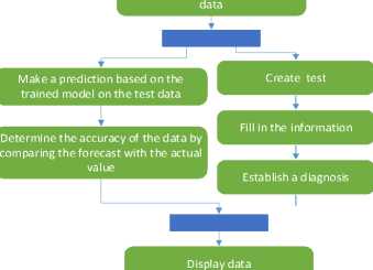
Fig.1. Activity diagram of the program's operation algorithm

After opening the test, we fill in all the information necessary for making a diagnosis. This action can be seen in more detail in Fig. 2. After filling in the information, the data verification process begins. We check whether there are answers to all the questionnaire questions and whether the numerical answers are entered correctly. If not all the fields are filled in, then we fill in all the fields or the age is filled in with other symbols (age is the only numerical field in our program), then we write the age in numbers and return to the data verification process. If the data verification is successful, that is, we fill in all the fields and the age is filled in with numbers, our trained program makes a diagnosis. At the end, the diagnosis and the accuracy of our program data are displayed on the screen. It completes the method.

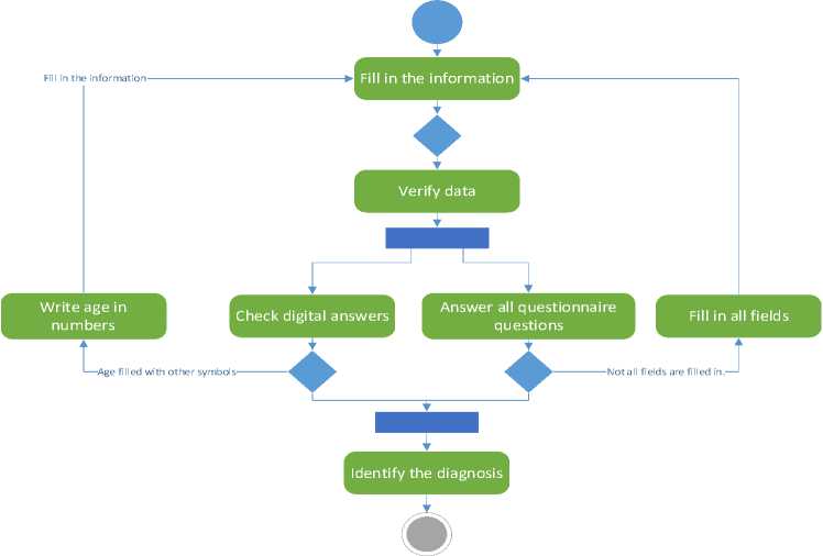
Fig.2. Activity diagram decomposition

Real-world pilot scenarios should be explored to evaluate the practical applicability of the proposed system in clinical settings. These may include integration with electronic medical records for continuous monitoring, deployment in family medicine clinics for primary screening, and patient-oriented mobile applications for self-assessment. Case studies in endocrinology clinics involving real patients can help validate the system's generalizability beyond the Pima Indian dataset and assess its behaviour with heterogeneous medical profiles.

Table 1. Real-world application scenarios and case studies for testing the system in a clinical setting

Name	Script	Purpose
Primary screening in family medicine	Family doctors use the system as a tool for pre-screening patients during annual check-ups. The patient enters basic clinical indicators (age, glucose level, BMI, blood pressure, etc.), and the system provides a probability of developing diabetes.	Identification of high-risk individuals. Referral of such patients for in-depth diagnostics (HbA1c analysis, glucose tolerance test).
Integration with electronic health records (EMRs)	Integration of the model with medical information systems in hospitals or clinics. The algorithm automatically analyses the patient's data updates and signals to the doctor about the increased risk.	Continuous monitoring of patients with prediabetic indicators. Warning the doctor about the need for preventive intervention.
Mobile application for patients at risk	Patients with obesity or a family history of diabetes install the app on their smartphone. They enter data on their own or through Bluetooth glucose meters/fitness trackers. The algorithm assesses the risk and provides recommendations.	Raising awareness of one's condition. Self-monitoring without regular visits to a doctor.
Case Study: Endocrinology Clinic	To attract 100 new patients with suspected diabetes to the clinic. Compare the decisions made by the system with the diagnoses of doctors. Measure accuracy, recall, false negatives, and user trust.	Discover how the model copes with different patient profiles. Determine how well it generalises outside of the Pima dataset.

The data from the Pima dataset is limited to one demographic group (women of the Pima tribe). Therefore, testing in real conditions with diverse populations will help assess the generalisation of the model. An assessment of the system's immunity to noisy or incomplete data is required, which often happens in real medical practice. Integration into clinical processes is an essential step towards real implementation.

We will describe the possibility of integrating glucose monitors with an AI-based diabetes prediction system in terms of technical details about how hardware and software interact, data synchronisation methods, and challenges associated with real-time data collection.

• •    Types of glucose monitors are traditional devices (with manual reading) and CGM systems (continuous glucose monitoring). Conventional devices are plugged into a USB or Bluetooth data transmission. CGM systems are devices that automatically record glucose levels every 5-15 minutes (for example, FreeStyle Libre, Dexcom).

• •    The ways to transmit data to the AI system are Bluetooth Low Energy (BLE), Wi-Fi / GSM modules, USB or NFC readers. BLE is the most common protocol for transmission to mobile applications. Wi-Fi / GSM modules are used in more advanced devices for direct synchronisation with cloud databases. USB or NFC reading is used for periodic manual data transfer to a computer

• •    Application interfaces are REST APIs from manufacturers (for example, Dexcom API), SDKs, or drivers for local data exchange (for example, via a COM port or Bluetooth socket). Also, program-by-program interfaces include the use of an intermediate data collection module, which receives and processes incoming streams and then transmits them to the AI module.

Data synchronisation methods include timestamp alignment, buffering, transmission confirmation mechanisms, flushing, and notification queues. Timestamp alignment — each data record contains an exact measurement time; The model synchronises records over time. Buffering - if data arrives intermittently, it is temporarily stored in a buffer until the whole block is processed. Acknowledgement mechanisms are data delivery confirmations that allow retransmission in case of loss. Logging and message queues — for example, via MQTT, RabbitMQ, or Kafka for reliable delivery and real-time processing.

Table 2. Potential problems with real-time data collection

Problem	Description	Potential consequence
Connection loss	Disappearing Bluetooth/Wi-Fi connection	Skipping measurements, incomplete data
Latency	Data arrives with a delay	Untimely decision-making
Anomalies/Outliers	Incorrect or noisy glucose values	False classification of the condition
Dependence on the device's battery	Turning off the device without warning	Monitoring interruption
Format incompatibility	Data from different devices has a different structure	The need for unification or conversion
Privacy and security	Transfer of medical data without encryption	Risk of personal information leakage

In the future, the system can be integrated with hardware glucose monitors, which will allow you to receive data in real time. Such integration involves the use of data transfer protocols (for example, Bluetooth LE or REST API), as well as intermediate modules for buffering and synchronising information with the AI software classifier. However, when working in real time, you should take into account potential risks such as connection loss, transfer delays, data outages, or privacy threats. For the stable operation of the system, it is necessary to implement mechanisms for retransmission, anomaly filtering, and ensuring the protection of medical data during transmission and storage.

Let us consider the financial aspects of the implementation of the diabetes prediction system, although this is an essential factor in the real implementation in medical practice. Below is a detailed analysis of the cost and resource requirements that should be considered when implementing such a system in a clinical setting.

Analysis of the cost of implementing a diabetes prediction system

• •    Hardware is continuous glucose monitors (CGMs), in particular, devices:

— FreeStyle Libre 2 / 3 (Abbott) — ≈ 80–150 USD / sensor (for 14 days);

- Dexcom G6 / G7 - ≈ 300-400 USD / starter kit, then 150-300 USD / month;

— Scanners/receivers — additional 100-200 USD (or using smartphones with NFC/Bluetooth).

The problem is the high regular cost for clinics with a large number of patients. Not all patients can afford the constant use of CGM at home. It is also necessary to certify the devices according to medical requirements.

• •    Computational resources for an AI model are based on model training. XGBoost, as a rule, does not require high computing power, but when working with larger sets (for example, >100 thousand records), there may be a need for GPU or cloud resources. The cost of using a GPU (e.g., on Google Cloud or AWS) is ≈ $0.50–$1.00/hour (GPU) and ≈ $0.10–$0.30/hour (CPU nodes). It can be implemented even on a regular server or a powerful laptop. Still, when processing data in real time (for example, from CGM), it is desirable to have a remote server or cloud infrastructure.

• •    Software infrastructure and support include:

— Cloud environment (AWS, Azure, GCP): ≈ 10-50 USD/month for the basic configuration;

- Patient databases (secure storage): ≈ 0.01–0.05 USD/GB/month;

— Integration with EMR (electronic medical records): requires separate APIs and legal compliance (HIPAA, GDPR).

• •    Additional costs are incurred for technical support, staff training and licensing/certification. In particular, for technical support, a system administrator or an IT specialist on the clinic staff is required. After training, doctors must understand how to interpret the results of the model. If the system will be used for clinical diagnostics, medical certification (CE, FDA, etc.) is required.

• 3.4.    Overview of Selected Datasets

Table 3. Potential barriers to implementation in medical institutions

Barrier	Explanation
High cost of CGM	Especially for chronic monitoring or mass adoption
Lack of infrastructure	Not all establishments have servers or stable Internet
Misunderstanding of AI Approaches	Distrust or misunderstanding on the part of doctors
Data privacy	The need to comply with medical data protection standards

One of the critical aspects that has not been addressed in this study is the cost of the practical implementation of the proposed system. Continuous glucose monitors (CGMs), which could provide real-world inputs to the model, have a relatively high cost for both patients and healthcare facilities. In addition, the implementation of the software part — including real-time data processing, storage of results, and interpretation of model conclusions — requires the availability of cloud infrastructure, secure databases, and technical personnel. These factors can become a serious obstacle to scaling the system in real clinical practice, especially in public institutions or countries with limited healthcare funding.

This section describes the key aspects of the dataset used to train and evaluate the model. The choice of dataset is determined by its representativeness, size, and relevance to the task at hand. Today, you can find a variety of datasets on the Internet that can be used to train machine learning models. The best resource is Kaggle, which not only allows you to access a number of tools and resources for research, study, and practice in the areas of data analysis and machine learning model development but also provides an excellent opportunity to participate in data science competitions, where participants from all over the world compete in solving real-world data collection and analysis problems. We have selected two datasets that we believe are best suited for training the model.

Table 4. Dataset characteristics

Data set	Number of characteristics	Number of records
1	9	768
2	9	100,000

The dataset contains attributes related to women's health. It includes the following attributes:

Pregnancies (number of pregnancies) affect the risk of developing diabetes, particularly gestational diabetes. Gestational diabetes is caused by insufficient insulin production or ineffective use of insulin by the body during pregnancy. This condition usually develops in the second trimester of pregnancy and may improve after delivery, but it can also increase the risk of developing type 2 diabetes later in life. The data type is integer. Thus, the frequency of pregnancies may be a risk factor through several mechanisms:

• •    Increased workload on the pancreas, particularly each new pregnancy, creates additional workload on the pancreas, which secretes insulin. The increased insulin load leads to exhaustion of the pancreatic beta cells.

• •    Metabolic changes, such as hormonal and metabolic changes, occur with every pregnancy. These changes affect the sensitivity of cells to insulin and may determine the development of insulin resistance.

Glucose (blood glucose level) shows the amount of sugar (glucose) in the blood at a given time. Glucose is the primary source of energy for the body's cells, and its regulation in the blood is essential for the body to function correctly. Blood glucose levels are measured in milligrams per deciliter (mg/dL) or millimoles per litre (mmol/L). Normal levels can vary depending on a number of factors, including the time of day and the time since you last ate. Changes in blood glucose levels can indicate a number of conditions, including diabetes, prediabetes, hyperglycemia (high glucose levels), and hypoglycemia (low glucose levels). Healthcare professionals can determine how high and low blood glucose levels are affecting your health and develop a strategy to treat or control these conditions. The data type is integer.

There are two types of Blood pressure. In our case, we use diastolic pressure (the lower number). Blood pressure is an essential indicator of the functioning of the circulatory system. It indicates the pressure exerted on the walls of the arteries by the blood circulating in the vessels. This pressure is determined by two numbers measured in millimetres of mercury (mm Hg). Systolic blood pressure (the higher number): reflects the maximum blood pressure in the arteries during the contraction of the heart, when blood is ejected into the vessels. Diastolic blood pressure (the lower number) reflects the lowest pressure in the arteries when the heart relaxes between heart contractions. For example, "120/80 mm Hg" means that the systolic pressure is 120 mm Hg and the diastolic pressure is 80 mm Hg. It is believed that normal blood pressure in adults is around 120/80 mm Hg. Changes in these values can indicate a number of conditions, including high blood pressure (hypertension), low blood pressure (hypotension), or other blood pressure problems that affect the cardiovascular system and overall health. Blood pressure assessment is an integral part of heart health and is considered in the diagnosis and treatment of cardiovascular disease. A data type is an integer.

Skin thickness is commonly measured in specific dimensions and can be used as one of many characteristics to determine diabetes risk and prognosis. However, it is not a direct indicator of diabetes in itself. There are several rationales for using skin thickness in the context of diabetes research. For example, the thickness of subcutaneous fat may be associated with insulin resistance, an essential factor in the development of type 2 diabetes. Insulin resistance means that the body's cells are less sensitive to insulin, which leads to increased blood glucose levels. However, skin thickness alone is not an accurate and reliable indicator of diabetes, and its use may be limited. The diagnosis of diabetes is usually made using specific tests, such as blood glucose levels and other biomarkers. Therefore, although skin thickness can be included in risk analysis and studies of the characteristics of people at high risk of diabetes, it cannot be the sole criterion for detecting diabetes. The data type is integer.

Insulin (insulin blood level) is a hormone secreted by the beta cells of the pancreas, an organ located behind the stomach, and is essential for regulating blood sugar (glucose) levels. The primary role of insulin is to regulate metabolism, especially that of carbohydrates. The data type is integer. The main functions of insulin in the body are:

• •    Lowering blood glucose levels, i.e. insulin, helps cells absorb glucose from the blood and reduces the concentration of glucose in the blood.

• •    Storing glucose in the form of glycogen, i.e. insulin, promotes the formation of glycogen - a form of glucose storage in the liver and muscles.

• •    Stimulating protein synthesis, i.e. insulin promotes the release of intracellular amino acids and facilitates protein synthesis.

• •    Accumulating fat, in particular, hormones, promotes the formation and accumulation of fat in cells.

• •    Inhibiting the breakdown of glycogen and fats, i.e. insulin maintains stable energy levels by inhibiting the breakdown of glycogen and fats.

• •    Beta-cell dysfunction and cellular insulin resistance can lead to metabolic disorders, including the development of type 2 diabetes, in which the body cannot use insulin effectively or cannot secrete enough insulin.

BMI (body mass index or weight-for-height ratio). Individuals with the highest BMI (mean 34.5 kg/m²) had an 11fold increased risk of developing diabetes compared to participants with the lowest BMI (mean 21.7 kg/m²). The group with the highest BMI had a higher probability of developing diabetes compared to all other BMI groups, regardless of genetic risk. Data type: floating point number.

DiabetesPedigreeFunction (Diabetes Pedigree Function) reflects the ratio of the number of people with diabetes to the total number of people in the family. Since the probability of acquiring diabetes during a person's life is very dependent on genetics, an indicator such as the number of people with this disease in the family should be taken into account. Data type: floating point number.

Age affects the risk of developing diabetes, especially type 2 diabetes. The data type is integer. The main ways in which age affects this risk are:

• •    Increased risk with age, in particular, the general trend is that the risk of developing diabetes increases with age. Statistics show that people over 45 have a higher risk of developing type 2 diabetes, and this risk increases with time.

• •    Metabolic changes, i.e. changes in metabolism, can occur with age, such as a decrease in the sensitivity of the body's cells to insulin. It leads to insulin resistance, which is an essential factor in the development of type 2 diabetes.

• •    Changes in body composition, for example, a woman's body can become larger with age, and the distribution of fat tissue can change. Being overweight and obese are risk factors for developing diabetes.

• •    Decreased physical activity, i.e. physical activity decreases with age, which can worsen insulin sensitivity and overall health.

Outcome, where 1 indicates the presence of diabetes, and 0 indicates the absence. The data type is binary (1 or 0).

This dataset is used to investigate factors that influence the development of diabetes in women, as well as to build machine learning models to predict the presence or absence of the disease. The balance and diversity of characteristics make this dataset an interesting topic for research and analysis. From the analysis of histograms of the distribution of the number of pregnancies among women, the following conclusions can be drawn:

• •    Most women have fewer than six pregnancies: many observations fall between 0 and 6 pregnancies, suggesting that most women in the study group have had relatively few pregnancies.

• •    The number of women with more than six pregnancies decreases significantly when the interval of six pregnancies is exceeded. It may indicate that there were more women with fewer pregnancies in this dataset, which is not surprising since most countries tend to reduce fertility.

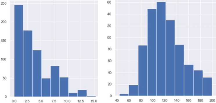
Fig.3. Distribution chart by age group in set 1 and by glucose level in set 1

From the analysis of the histograms of the distribution of the number of women by blood glucose level, the following conclusions can be drawn:

• •    Most women have normal blood glucose levels. According to the general distribution, most women have blood glucose levels within the normal range of 79.6 to 119.4. The number of women in these ranges (156 and 211, respectively) is significant.

• •    The proportion of women with low or high glucose levels is small. The study shows that very few women have glucose levels below 19.9 or above 199. This distribution suggests that extreme glucose levels are rare in the study group.

• •    Based on the analysis of the histogram of the distribution of the number of women by blood pressure reduction, the following conclusions can be drawn:

• •    Most women have normal blood pressure levels. The general distribution shows that most women have blood pressure within the normal range (61-97.6). This range is the zone of normal blood pressure, and the number of women in this range is significant (87-261 women).

• •    Very few women have low and high blood pressure. Blood pressure ranges of less than 24.4 and more excellent than 109.8 are rare in the study population. It suggests that extreme hypotension is rare in the study population.

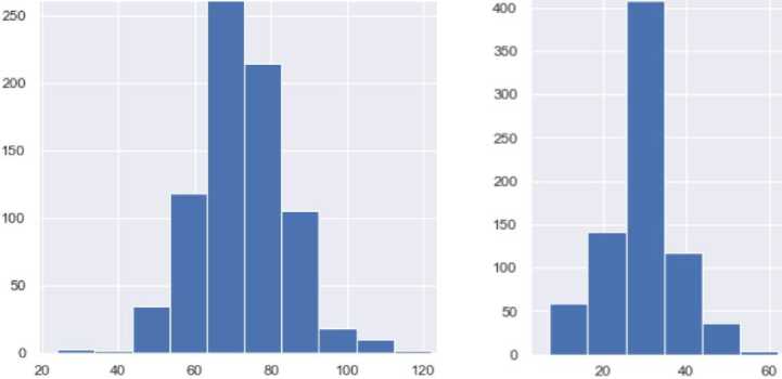
Fig.4. Distribution diagram by lower blood pressure level in set 1 and by skinfold thickness level in set 1

From the analysis of histograms of the distribution of the number of women by skin thickness, the following conclusions can be drawn:

• •    Most women have skin thickness within the normal range. According to the general distribution, most women have skin thicknesses within the normal range of 9.9 to 49.5. The number of women in this range is vast.

• •    Very few women have very thin or very thick skin. The ranges of skin thickness below 9.9 and above 59.4 are small in the study population. It indicates that extreme values of skin thickness in the study population are rare.

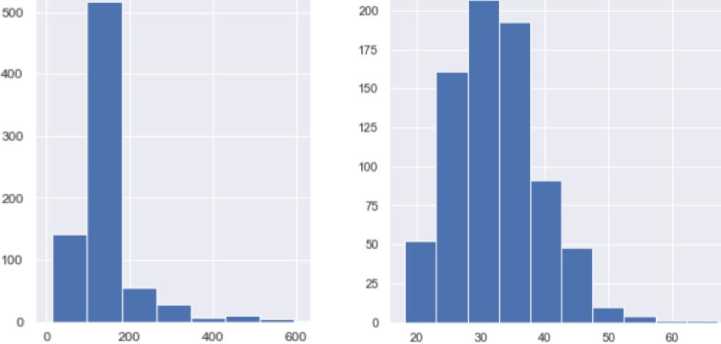
Fig.5. Distribution chart by insulin level in set 1 and by BMI level in set 1

Based on the analysis of the histogram of the distribution of the number of women depending on the insulin level, the following conclusions can be drawn:

• •    Most women have low insulin levels. According to the general distribution, most women have low insulin levels since a significant peak in the number of women is observed in the range from 0 to 84.4. It may indicate that most of the study participants have normal insulin levels.

• •    Fewer women with moderate insulin levels. The insulin range of 84.6 to 169.2 has fewer women compared to the low range. It may indicate that those with moderate insulin levels are underrepresented.

• •    Based on the analysis of the histograms of the distribution of the number of women by body mass index (BMI) levels, the following conclusions can be drawn:

• •    Distribution of women with different BMI values. The histograms show the distribution of women with different BMI values. The BMI of the majority of the study participants ranged from 20.1 to 33.5, which is the range between normal and overweight, according to the World Health Organization (WHO).

• •    Peaks in the standard and overweight range. There are peaks in the standard (26.833.5) and overweight (20.126.8) ranges. It may indicate that participants with these BMI values are more common in this study.

• •    Few women with extreme BMI values. The small number of BMI values in the ranges below 20.1 and above 40.2 suggests that there were few participants with low and high BMI values in this study.

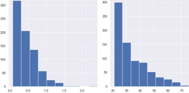
Fig 6. Diagram of the family sample of diabetes in set 1 and by age in set 1

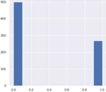
Fig.7. Distribution chart by score in set 1

Based on the analysis of histograms of the distribution of the number of women by DiabetesPedigreeFunction level, the following conclusions can be drawn:

• •    Overall distribution by DiabetesPedigreeFunction. The histograms show the distribution of women across different ranges of DiabetesPedigreeFunction values. Most of the study participants have DiabetesPedigreeFunction values between 0 and 0.3.

• •    Fewer women have high DiabetesPedigreeFunction values. Very few women have values above 0.55 (inclusive), indicating that high DiabetesPedigreeFunction values are not very common in the study population.

• •    A small proportion of women with very high or very low function values. The proportion of women in the ranges above 1.25 and below 0.3 is small, indicating that the number of women with very high or very low diabetes function values due to heredity is limited.

After reviewing the datasets, you should start building an AI model. To design the model, we will use the Google Colab service, which uses Jupyter Notebooks. They can be used to run and develop Python code in a cloud environment; a significant advantage of Google Colab is free access to high-performance graphics processing units (GPUs) and tensor processors (TPUs), which can be used to accelerate AI tasks (for example, training neural networks). To create a model, you should first decide on a set of libraries that will help in writing this project. The following were selected: Matpotlib, Seaborn, Pandas, Numpy, Missingno, and Sklearn.

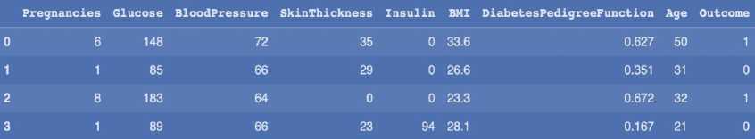
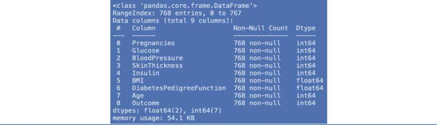
	Pregnancies	Glucose	BloodPres sure	SkinThickness	Insulin	BMI	DiabetesPedigreeFunction	Age	Outcome
count	768.000000	768.000000	768.000000	768.000000	768.000000	768.000000	768.000000	768.000000	768.000000
mean	3.845052	120.894531	69.105469	20.536458	79.799479	31.992578	0.471876	33.240885	0.348958
std	3.369578	31.972618	19.355807	15.952218	115.244002	7.884160	0.331329	11.760232	0.476951
min	0.000000	0.000000	0.000000	0.000000	0.000000	0.000000	0.078000	21.000000	0.000000
25%	1.000000	99.000000	62.000000	0.000000	0.000000	27.300000	0.243750	24.000000	0.000000
50%	3.000000	117.000000	72.000000	23.000000	30.500000	32.000000	0.372500	29.000000	0.000000
75%	6.000000	140.250000	80.000000	32.000000	127.250000	36.600000	0.626250	41.000000	1.000000
max	17.000000	199.000000	122.000000	99.000000	846.000000	67.100000	2.420000	81.000000	1.000000

Fig.8. The first 4 data from dataset 1, information about dataset attributes and detailed information about the dataset

Table 5. Description of selected libraries

Library	Description	Using
Matplotlib (import matplotlib.pyplot as plt)	It is a graphing and data visualization library for Python. It provides extensive functionality for creating various types of graphs, from line graphs to histograms and contour plots.	Data visualization, dependency exploration, and creation of attractive graphs
Seaborn (import seaborn as sns):	It is a high-level data visualization library based on Matplotlib. It adds layers of abstraction and provides styling and high-level functions for quickly creating stylish plots.	It should be used to create attractive graphs and data visualizations.
Pandas (import pandas as pd):	It is a library for data processing and analysis; it provides data structures such as DataFrame and allows you to efficiently work with tabular data; with Pandas, you can easily process and analyze large amounts of data.	Used to load, process, and analyze data, especially in the form of tabular structures.
NumPy (import numpy as np):	It is a computational mathematics library used in Python. It provides high-performance arrays and operations on them, allowing you to easily process numerical data.	It supports operations on arrays, vectors, and matrices and is very useful for scientific computing and data processing.
missingno (import missingno as msno):	It is a library for visualizing missing values in a dataset. It allows you to quickly estimate the number and location of missing data in the form of matrices and graphs.	Used during the data analysis phase to detect and visualize missing values.
sklearn (from sklearn import metrics)	A machine-learning library for Python that contains various algorithms for classification, regression, clustering, and other machine-learning tasks. In this case, its metrics submodule is imported, which includes multiple metrics for evaluating the quality of machine learning models.	It is used to evaluate the performance of machine learning models to calculate metrics such as accuracy, repeatability, and F1 metrics.

To ensure transparency and reproducibility of the study, we will indicate which approaches, specific methods, algorithms and tools were used at the stages of data preprocessing, in particular during normalisation and processing of missing values. Detailed description of data preprocessing methods:

Processing missing values (imputation). In a preliminary analysis of the dataset, it was found that some features, although not formally containing empty values (NaN), have unrealistic null values, actually reflecting omitted or unrecorded data (e.g., zero glucose, insulin, skin thickness, etc.). Such values were replaced using the median imputation method. For each trait with "suspicious" zeros, the median was calculated based on only non-zero values. All zero values in this sign have been replaced with the corresponding median. This approach is chosen because of its tolerance to emissions, especially in data with an asymmetric distribution (e.g., insulin).

for column in ['Glucose', 'BloodPressure', 'SkinThickness', 'Insulin', 'BMI']:

median = df[df[column] != 0][column].median()

df[column] = df[column].replace(0, median)

Normalisation (scaling of features). To ensure the correct operation of machine learning algorithms that are sensitive to data scale (for example, k-NN or SVM), Z-normalisation (standardisation) is applied. Each numerical feature is transformed in such a way as to have a mean of 0 and a standard deviation of 1. To do this, we used the StandardScaler tool from the scikit-learn library. This approach is appropriate because most of the features in the dataset have a roughly normal distribution.

from sklearn.preprocessing import StandardScaler scaler = StandardScaler()

We will connect Google Drive to Google Colab using the drive.mount() command. It will allow us to access the files stored on it. In our case, these are dataset files. After completing these steps, our Google Drive will be available in the /content/drive folder in the Colab environment, and we will be able to easily access the files in Google Drive from our code. We will get information about each of the attributes of the dataset: the column number, its name, the number of rows, and the data type of the column. Now, let's review detailed information about each of the attributes: the number of values, the minimum value, the maximum value, and the arithmetic mean. First, let's divide the dataset into attributes indicating health indicators and labels determining the presence or absence of diabetes. Scaling of the input features should be performed to optimize and speed up model training. It is also important to level the influence of large values, which can dominate and overlap the influence of much smaller values. The main goal of scaling is to bring attributes to a common scale. There are several types of scaling, all of which are available in the sclearn library:

Normalization (Min-Max Scaling) brings the values of the input features to the interval from 0 to 1, where 0 is the most significant value in the column, and one is the largest. This type of scaling is usually used when the absolute value of the features is important to us and when it is uneven.

Standardization (Z-Scope Scaling) brings the values of the input features to the interval with a mean value of 0 and a standard deviation of 1, i.e. each attribute value is the ratio of the difference between its value and the column mean to the standard deviation of the feature. This type of scaling is used when the distribution of the feature values is normal.

In our case, standardization will be used since the distribution of features is normal. Now, we need to divide the data available in the dataset into data that we will use for training and testing. We need them in order to check the accuracy of the model after training. For division, we will use the test_train_split function from the sklearn.model_selecting library:

• •    Splitting the dataset into training and tests is essential for evaluating the performance of machine learning models on unknown data.

• •    Features and target variables are passed, the size of the test set (or training set) is specified, and, if necessary, a random value is set for repeatability. The function returns four sets: training features ( x_train ), test features Strain ), training target values (x_test ), and testing target values (y_test ).

We will use several machine learning methods, namely Random Forest, Decision Tree, and Support Vector Machine. Then, we will compare their accuracy and choose the one that best suits our problem.

standard_scaler_X = StandardScaler()

X= pd.DataFrame(standard_scaler_X.fit_transform(X), columns= ['Pregnancies', 'Glucose',

' BloodPressure', 'SkinThickness',

'Insulin', 'BMI1,

]'DiabetesPedigreeFunction', 'Age'])

X.headO

	Pregnancies	Glucose	BloodPressure	SkinThickness	Insulin	BMI	DiabetesPedigreeFunction	Age
0	0 639947	0.848324	0.149641	0.907270	-0.692891	0.204013	0.468492	1.425995
1	-0.844885	-1.123396	-0.160546	0.530902	-0.692891	-0.684422	-0.365061	-0.190672
2	1.233880	1.943724	-0.263941	-1.288212	-0.692891	-1.103255	0.604397	-0.105584
3	-0.844885	-0.998208	-0.160546	0.154533	0.123302	-0.494043	-0.920763	-1.041549
4	-1.141852	0.504055	-1.504687	0.907270	0.765836	1.409746	5.484909	-0.020496

Fig.9. Example of scaling and its result

Table 6. Description of machine learning methods

Name	Type	Description
Random Forest	Ensemble	It is a decision ensemble that uses many decisions (decision trees) to make predictions. Each tree computes a prediction, and the final prediction of this method is made by summing the projections of all the trees. An important feature is that each tree is built on a random subset of the data and only takes into account a subset of specific features, which helps reduce overfitting and increase the reliability of the model.
Decision Tree	Classification or regression	Decision trees are structured as a tree, where each node divides a data sample along a specific feature. Each leaf of the tree corresponds to a final class (in the case of classification) or a number (in the case of regression). Nodes are divided according to criteria such as entropy or Gini coefficient. Decision trees are straightforward to interpret, but they are very prone to one common problem encountered in ML: overfitting.
Support Vector Machine	Classification or regression	The support vector method creates a hyperplane that maximally separates classes. The vectors on the solution boundary are called support vectors. Models created using this method have great power when dealing with high-dimensional data and generalize well to the data. The vital point is the choice of an appropriate kernel function, which determines how the distances between points in space are measured.

First, we will create a model that uses the Random Forest method. We import the corresponding method from the sklearn library. When initializing the methods, we need to specify the number of trees that will be created for training (n_estimators). Then, we pass the input features (x_train) and labels. After training the model, we should check the accuracy of the model both on the data on which it was trained and on the data that was missing. To do this, we will need the accuracy_score function, which checks whether the prediction matches the truth and calculates the corresponding accuracy percentage - 0.7637795275590551. We can see that this model has relatively high accuracy rates both on the data set on which training took place and on the data that was previously set aside for testing, namely 100% and 76% accuracy, respectively. Now, we will create a model that uses the Decision Tree method. Let's check the accuracy of this model (0.6968503937007874). Finally, we will create a model that uses the Support Vector Machine method. Let's check the accuracy of this model (0.7519685039370079). It is easy to see that the accuracy of this method, when tested on the data it was trained on, has significantly decreased compared to previous methods.

4.    Experiments 4.1.    Data Pre-processing and Results Presentation

• •   https://www.kaggle.com/datasets/kevintan701/diabetes-prediction-datasets

• •   https://www.kaggle.com/datasets/uciml/pima-indians-diabetes-database

  user id	date	weight | height	blood glucose | physical activity | diet	medication adherence	stress level	sleep_hours	hydration level bmi		risk score
  1	2021-01-01	77,45071 183,9936	112,992869            0            1	0	1	6,342317383	1          22,9		38
  2	2021-01-02	67,92604 179,2463	134,2192532      12,79229978       0	1	2	10,65812162	1	21,1	39,16231
  3	2021-01-03  79,71533 170,5963		108,3032032      21,72788933       1	1	0	5,997831759	1	27,4	31,48163
  4	2021-01-04 92,84545 163,5306		127,6815388      67,75375315       1	0	1	7,958813835	1	34,7      45
  5	2021-01-05   66,4877 176,9822		70           41,13106249       1	1	0	6,774707366	1	21,2   4,717234
  6	2021-01-06 66,48795 173,9349		148,5317483      3,290368618       0	1	0	7,901650629	0	22	32,01289
  7	2021-01-07 93,68819 178,9519		140,048219       39,72072579       1	1	2	8,673951745	1	29,3	30,06982
  8	2021-01-08 81,51152 176,3517		107,3164548           0            1	1	0	6,292043013	1	26,2	33
  9	2021-01-09  62,95788 180,4955		166,3698267      51,65382108       0	1	0	8,419546853	1	19,3	12,08654
  10	2021-01-10	78,1384 164,6476	177,5028055      20,57750696       0	1	1	12	1	28,8	46,82675
  11	2021-01-11	63,04873 183,1739	75,69760543      28,12727623       1	1	0	8,135079988	1	18,8	9,561817
  12	2021-01-13	63,01405 171,976	109,4910089      56,51593295       0	0	2	10,22716293	1	21,3	40,87102
  13	2021-01-14	73,62943 190,7526	109,234306       4,256728628       0	0	2	7,962092	1	20,2	51,72298
  14	2021-01-15	41,3008 163,1081	102,403876       2,057636298       1	1	2	5,136076756	1		42,38271
  15	2021-01-16	44,12623 187,3596	173,1789937      18,32801347       1	1	o	7,551387995	1	12,6	22,5016

Fig.10. Fragment of the reporting table

Consider the critical aspects of the Pima Indians Diabetes dataset among the many other medical datasets available (e.g., NHANES, MIMIC-III, etc.), including its limitations. In the Pima Indians Diabetes set, there is a significant imbalance between the number of sick and healthy ones (the number of negative examples exceeds the number of positive ones). It may affect accuracy, in particular recall and F1 estimation, but the authors do not mention whether this was taken into account during the simulation (e.g., by using data balancing methods — SMOTE, oversampling, etc.). The data were collected exclusively among women from the Pima Indian tribe, which seriously limits the environmental validity of the model. It means that the results of the model can hardly be transferred to other ethnic groups or men. This aspect is not mentioned, although it is a significant weakness in terms of using the results in a global context, which is stated in the title of the work ("... in the world").

The Pima Indians Diabetes Dataset was chosen because of its free availability, historical significance in diabetes-related research, and an exhaustive list of clinically relevant attributes. However, we are aware of its limitations — in particular, the imbalance of classes and the fact that all records relate to women from the same ethnic group. It limits the model's ability to generalise the results to a more heterogeneous population. In the future, broader and more representative datasets will be used to increase the versatility of the developed system. The main reasons for choosing:

• •    Open accessibility and structure, because the dataset is open and easily accessible, particularly through the Kaggle platform. It is well-structured, containing 768 records with nine clinical parameters, allowing you to quickly prepare data for machine learning without the need for complex pre-cleaning.

• •    Practical orientation of the attributes, because all the characteristics of the dataset (for example, glucose level, blood pressure, body mass index, number of pregnancies, etc.) are clinically relevant, which allows you to build a predictive model focused on fundamental risk factors for diabetes.

• •    Wide recognition in the scientific community, as this set is often used as a standard for comparing the effectiveness of different machine learning models, which makes the results of the study more comparable with other works in the field.

At the same time, a number of essential restrictions should be noted:

• •    Limited demographic sample, since the data are collected exclusively among women from the Pima tribe, which does not allow generalising conclusions to other ethnic or gender groups.

• •    Class imbalance in the sample, since the number of patients without diabetes significantly exceeds the number of patients with diabetes, which may affect the accuracy of the model without additional measures (for example, resampling).

• •    The limited size, in particular, the relatively small number of records (768), reduces the potential for deep analyses or working with more complex neural network models.

Despite these limitations, Pima Indians Diabetes was chosen as a starting point for modelling due to its convenience, practicality, and representativeness of key medical indicators. In the future, the study will be expanded with the help of more representative and modern medical datasets to increase the generalisation of the model.

The study used the Pima Indians Diabetes dataset, which contains records of only women over the age of 21 from one ethnic group — the Pima Indians tribe. Let's analyse the possible biases and limitations that arise when trying to generalise the results of the model to other populations.

Potential biases and limitations when generalising the model to other populations

• •    Limited demographic representativeness consists mainly of the fact that all data are obtained from women from the Pima tribe in Arizona, USA. The model does not include men, members of other races or ethnicities (African Americans, Europeans, Asians, etc.), and patients with other eating or cultural habits. The model could potentially not work correctly when applied to wider, more diverse populations, due to differences in genetics, lifestyle, and access to care.

• •    The risk of demographic bias is that attributes that have diagnostic value for one group (e.g., BMI, insulin levels) may have a different impact in other populations. Neural networks or decision trees trained on such data can

automatically "learn" to reinforce bias (e.g., underestimate risk in men or children).

• •    Cultural and behavioural differences affect the incidence of diabetes, as well as the manifestations of symptoms. They may depend on food intake (carbohydrates, fats), level of physical activity, and access to health education and prevention. A model built on data from a specific environment can incorrectly classify individuals from other social and economic conditions.

• •    Overestimation of accuracy when transferring the model is one of the significant biases. In particular, even if the model has high accuracy on Pima data, this does not guarantee its effectiveness on wider medical bases such as NHANES, MIMIC-III, etc. It is because the model may not be able to generalise well to new patterns that it did not see during training.

One of the critical limitations of this study is the use of the Pima Indians Diabetes dataset, which covers only women of a particular ethnic group. It creates a potential risk of demographic bias in the model when applied to wider populations with different ethnic, social, and cultural backgrounds. Indicators that are critical predictors for one population may have a different meaning for others. In further research, it is advisable to test the model on more representative and diverse data sets in order to assess its generalizability and adapt it to the needs of a broader range of users.

The graphs show the relationships between glucose levels and physical activity and between risk factors and weight. The first graph illustrates the dispersion of blood glucose levels depending on the level of physical activity. There is a weak or almost no relationship between these parameters. Glucose values vary significantly in the range from 50 to 300, regardless of the level of physical activity. Most of the points are concentrated near low activity values, which may indicate a predominantly sedentary lifestyle among the subjects studied. It emphasizes that physical activity alone is not the key factor determining glucose levels, but its influence may be manifested in combination with other factors, such as weight or diet.

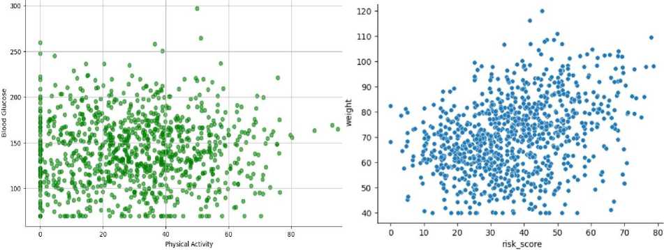
Fig.11. Diagram of the dependence of glucose level on physical activity in the Cartesian coordinate system and the dependence of the disease risk indicator on weight in the Cartesian coordinate system

The second graph shows the relationship between risk score and weight. There is a moderate positive correlation here, with increasing weight increasing risk. Most of the data is concentrated in the weight range of 60 to 90 kg and risk score of 20 to 50, indicating a typical profile for the individuals studied. However, there are some cases with high-risk scores even at relatively low weights, which may indicate other important risk factors, such as age, genetics, or comorbidities. It shows the need for further analysis to identify weight thresholds that significantly increase risk. The selected graphs were selected from among the other options because they showed more pronounced relationships, while the other graphs showed much more scattered data. They allow us to assess trends and highlight potential relationships, making them useful for further research. The first graph emphasizes the need to consider the complex influence of factors such as diet and stress, while the second confirms the importance of weight control in reducing risk scores. Further steps include conducting cluster analysis to group the data, building regression models to quantify the relationships, and testing hypotheses about the multifactorial influence on the studied indicators. It will help formulate specific recommendations for risk prevention and health management. Activity and glucose plots show the relationship between physical activity and blood glucose levels in polar coordinates. Each point represents a specific combination of activity and glucose levels. The points are concentrated predominantly in one sector, indicating the particular range of activity and glucose levels that prevail in the study sample. The distance of the points from the centre indicates the glucose level, while the angular coordinates reflect physical activity. This graph shows that most of the points are clustered in the low-activity range. Glucose levels often exceed 100 and even reach 300, which may indicate that low physical activity is a potential risk factor for high blood glucose. The data suggest the need for further research into the relationship between these indicators to confirm or refute the effect of activity on sugar levels. This graph highlights the need to encourage physical activity as a tool to reduce the risks associated with high glucose levels.

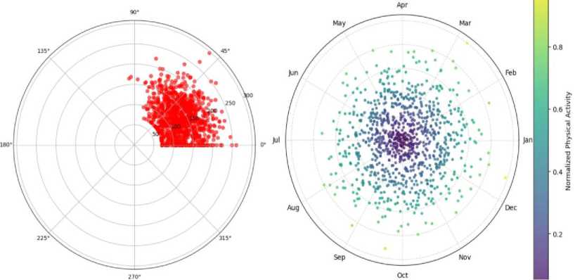
Fig.12. Diagram of the dependence of the activity indicator on the glucose level in the polar coordinate system and the cyclicity of physical activity in the polar coordinate system

The physical activity cycle diagram illustrates the cyclical nature of physical activity throughout the year in a polar coordinate system. Each point corresponds to a specific level of physical activity, normalized to a value between 0 and 1, and displayed in colour. The angles on the graph correspond to the months of the year (January is 0°, December is 360°), which allows us to assess seasonal trends. This graph clearly shows the seasonal, cyclical nature of physical activity. There is an increase in activity during the warmer months (spring-summer), while the winter months show a decrease in activity. The concentration of points closer to the centre during cold periods indicates a reduction in physical activity during this time. The highest levels of activity are seen in the summer months, which may be related to better weather conditions and increased motivation to engage in sports or outdoor activities.

Описова	статистика: user_id      weight      height blood_glucose physical_activity
mean std min	500.500000   70.361797  170.795375     140.818899          30.294497 288.819436   14.467165    9.742934      38.064177          19.305165 1.000000   40.000000  150.000000      70.000000           0.000000
max cv (%)	1000.000000 120.000000 200.000000     297,049508          94,861859 57.706181   20.561108    5.704449      27.030588          63.724991 diet medication_adherence stress_level sleep_hours \
mean std min	0.604000              0.693000      0.950000     7.076312 0.489309              0.461480      0.833183     1.883829 0,000000                0,000000      0,000000     4.000000
max cv (%)	1.000000                1.000000      2.000000    12.000000 81.011445             66.591658     87.703492    26.621621 hydrationlevel       bmi riskscore
mean std min	0.710000  24.385500   36.422120 0.453989   5.872022   14.898022 0.000000  10.900000    0.000000
max cv (%)	1.000000 45.200000   78.745396 63.942127 24.079973   40.903774

	user_id	weight	height	blood_glucose	physical_activity	diet	medication_adherence	stresslevel	sleep_hours	hydration_level	bmi	risk_score
mean	500.500000	70.361797	170.795375	140.818899	30.294497	0.604000	0.693000	0.950000	7.076312	0.710000	24.385500	36.422120
std	288.819436	14.467165	9.742934	38.064177	19.305165	0.489309	0.461480	0.833183	1.883829	0.453989	5.872022	14.898022
min	1.000000	40.000000	150.000000	70.000000	0.000000	0.000000	0.000000	0.000000	4.000000	0.000000	10.900000	0.000000
max	1000.000000	120.000000	200.000000	297.049508	94.861859	1.000000	1.000000	2.000000	12.000000	1.000000	45.200000	78.745396
cv(%)	57.706181	20.561108	5.704449	27.030588	63.724991	81.011445	66.591658	87.703492	26.621621	63.942127	24.079973	40.903774

Fig.13. Descriptive statistics table

The diagram in Fig. 12a indicates a possible relationship between low physical activity and elevated glucose levels, which emphasizes the importance of an active lifestyle for metabolic control. The diagram in Fig. 12b demonstrates seasonal fluctuations in activity, which is helpful for planning preventive measures aimed at maintaining regular training even during periods of reduced activity. Both diagrams complement each other, allowing for a comprehensive assessment of the role of physical activity as a factor influencing health. The results of descriptive statistics reflect the main quantitative characteristics of the data set, which include indicators of weight, height, glucose levels, physical activity, diet, medication intake, stress levels, sleep duration, hydration levels, body mass index (BMI), and risk. The average blood glucose level is 140.82, with a minimum value of 70 and a maximum of 297. The high coefficient of variation (27.03%) indicates significant variability in this indicator among the study participants. The average level of physical activity is 30.29. Still, the standard deviation (19.31) and coefficient of variation (63.72%) indicate significant differences in activity levels between respondents - some have zero activity, while others have more than 94.86.

The mean values for dietary discipline (0.60) and medication adherence (0.69) indicate that participants generally demonstrate moderate adherence to a healthy lifestyle. Still, the high variability of these indicators (81.01% and 66.59%, respectively) indicates significant differences in behaviour. Stress levels have a mean value of 0.95 with a substantial standard deviation (0.83), confirming high fluctuations among participants, with some reaching a maximum stress level of 2 points. Hydration averages 0.71, which is relatively high, but the coefficient of variation of 63.94% shows significant deviations from the mean. Body mass index (BMI) averages 24.39, which is within the normal range, although maximum values (up to 45.2) indicate obesity. The risk score has an average value of 36.42, but significant variability (40.90%) shows a wide distribution of data from zero to almost 79 risk points.

Overall, descriptive statistics indicate a wide range of values for most parameters, indicating sample heterogeneity. High coefficients of variation for physical activity, stress level, medication use, and diet highlight the importance of further analysis to identify risk groups and establish relationships between health factors. These results allow us to identify key indicators for predicting health status and optimizing preventive measures. The first histogram in Fig. 14 shows the distribution of blood glucose levels among the subjects. The majority of values are in the range of 100–160, with some cases of elevated levels up to 297. The distribution is skewed to the right, which may indicate the presence of a group of people with elevated glucose levels, potentially at risk for diabetes or other metabolic disorders. This graph allows us to estimate the prevalence of abnormal values and to determine the typical limit of expected values.

The second histogram shows the distribution of body mass index (BMI). The majority of the values are in the range of 20–30, which corresponds to normal and overweight body weight. There is also a group of individuals with a BMI above 35, which indicates the problem of obesity among some of the subjects. The histogram demonstrates an approximation to a normal distribution with a slight asymmetry to the right, confirming that a significant part of the sample is at risk of metabolic disorders due to being overweight.

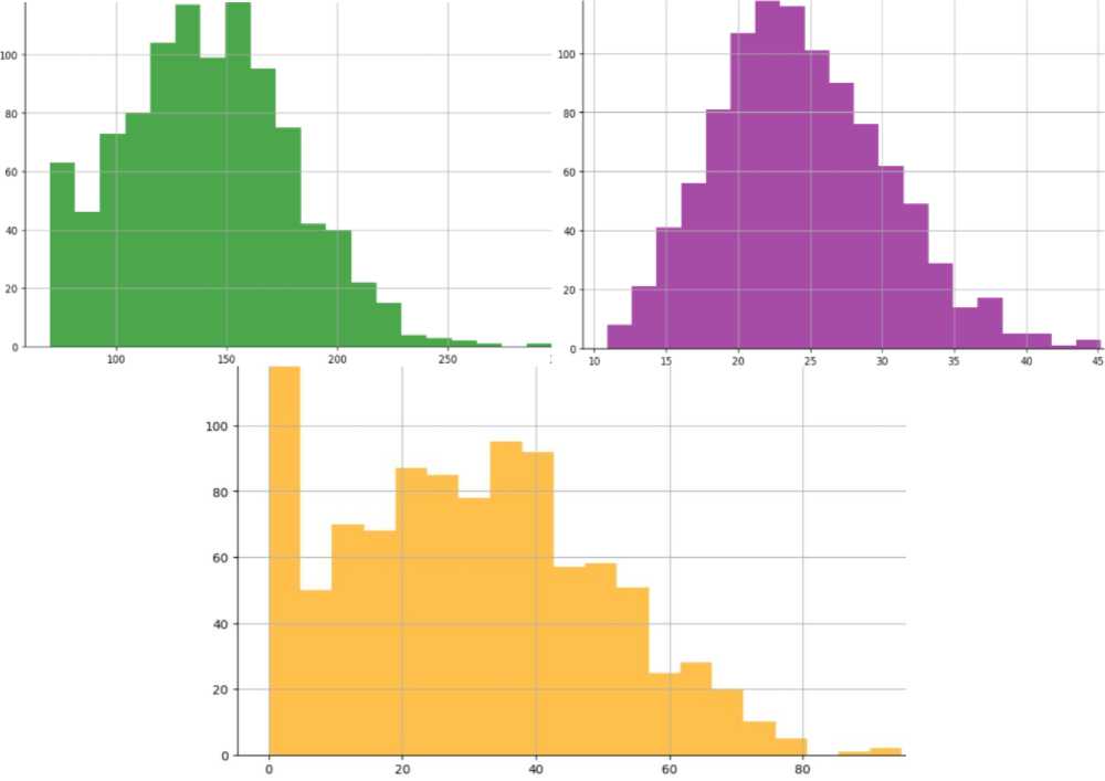
Fig.14. Histogram of blood glucose levels, body mass index and physical activity

The third bar graph illustrates physical activity levels. The data is strongly skewed to the left, with the most significant proportion of people showing very low levels of physical activity (0 to 20 minutes). A small number of people show higher levels of activity, highlighting the general trend towards a sedentary lifestyle. It may be an essential factor in the increased risk of metabolic diseases and supports the need to encourage physical activity to improve health.

These histograms provide information about the main risk factors among the sample – elevated glucose levels, overweight, and insufficient physical activity. They allow for the identification of risk groups and provide the basis for further analysis of the relationships between these indicators and the development of preventive measures.

In Fig. 15a, the graph shows the accumulated frequency of glucose levels. The X-axis shows the glucose level, and the Y-axis indicates the number of observations with glucose levels below a specific value. The accumulated frequency increases in steps, corresponding to the intervals of the histogram. The graph indicates that most values are in the range of 70–200, and only a small number of observations exceed 250. It is helpful in estimating the absolute number of cases with glucose levels below a specific value and confirms that the bulk of the sample exhibits moderate glucose levels.

In Fig. 15b, the graph shows the cumulative distribution of blood glucose levels as the probability that a value does not exceed a certain level. The horizontal axis shows glucose levels, and the vertical axis shows the cumulative probability. The curve rises smoothly from 0 to 1, indicating a uniform increase in likelihood with increasing glucose levels. Most values are in the range up to 200, after which the curve flattens out, showing saturation. It indicates that a significant proportion of observations have glucose levels below this threshold, and very high values are rare. The cumulant helps estimate the probability that glucose levels fall within a specific range; for example, 80% of values are less than 200. So, the second cluster allows you to analyse the data in terms of probability, and the first one is through the absolute frequency of occurrence. Together, they give a more complete picture of the distribution of glucose levels, helping to understand how common high values are and assess the risks of elevated glucose levels.

Smoothing with Kendall formulas:

• •    smooth the data using the smoothing interval sizes w = 3, 5, 7, 9, 11, 13, 15. We should get seven columns in a row;

• •    smooth the data using the smoothing interval size w = 3, then smooth the obtained smoothed data again, but use the smoothing interval size w = 5. We continue smoothing the received data with the smoothing interval w = 7 and so on until w = 15. We should get seven columns in a row.

• •    in both cases, find the number of turning points and the correlation coefficients between the original and smoothed values for each smoothing.

  

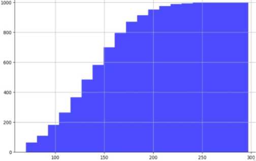
  Fig.15. Glucose level cumulation (by histogram data) and glucose level cumulation (by integral percentage)

  
  
  
  
  

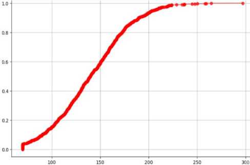
0

3

1000

0.570344

0

5

1000

0.476680

1

5

1000

0.429182

1

7

1000

0.378913

2

7

1000

0.350771

2

9

1000

0.326795

3

9

1000

0.304948

3

11

1000

0.302161

4

11

1000

0.288454

4

13

1000

0.288767

5

13

1000

0.279572

6

15

1000

0.268529

5

15

1000

0.269615

The graphs and tables show the results of smoothing glucose levels using Kendall's formulas, which allow you to remove fluctuations and identify general trends in the data. The first graph illustrates the results of individual smoothing for intervals from 3 to 15, where increasing the interval reduces fluctuations, making the graph smoother. Smaller intervals (w=3, 5) better reflect local fluctuations, while larger ones (w=11, 13, 15) suppress small volatility, focusing on global trends. The second graph shows repeated smoothing with increasing intervals, starting at three and gradually rising to 15. This approach provides even stronger smoothing, effectively removing noise but reducing detail.

The tables detail the results of the analysis, showing the number of turning points and the correlation coefficients between the original and smoothed data. In the case of single smoothing (point a), the correlation coefficients decrease with increasing intervals, indicating the loss of local fluctuations and smoother averaging. Repeated smoothing (point b) also shows a decrease in correlation. Still, the initial correlation values are higher due to the increase in intervals, which gradually dampens noise and improves visual smoothness. The graphs and tables emphasize that the choice of interval and smoothing method depends on the objectives of the analysis. Smaller intervals are better suited to detecting shortterm changes, while larger ones provide a clearer picture of long-term trends. The results allow us to compare the two methods and determine the optimal balance between detail and smoothness for a particular study.

The first graph in Fig. 18 shows the results of separate smoothing using Pollard formulas with fixed intervals from 3 to 15. It illustrates how, with increasing intervals, the variability decreases, and the graphs become smoother. However, large intervals lead to the loss of local fluctuations and simplification of the data, which can be seen when moving from small (w=3, 5) to larger (w=13, 15) intervals. The second plot in Fig. 18 shows repeated smoothing with increasing intervals. Starting at interval 3, the resulting smoothed data is smoothed again with larger intervals up to 15. This approach provides stronger averaging, which effectively reduces noise but also muffles details even more than in the first plot.

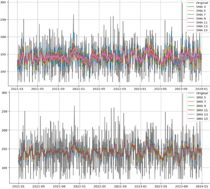
Fig.16. Smoothing for different intervals and repeated smoothing with increasing intervals

Fig.17. Table of smoothing results with intervals, turning points and correlation

The tables in Fig. 19 contain the results of the analysis, including the number of turning points and the correlation coefficients between the original and smoothed data. In both cases, the number of turning points remains stable (1000), indicating that the underlying structure of the data is preserved, but the correlation coefficients decrease with increasing intervals. It shows a gradual loss of similarity to the original data due to the stronger smoothing. The initial coefficients in the Pollard method are higher than in the Kendall method, indicating less loss of detail, especially for small intervals. The results of the analysis allow us to evaluate the effectiveness of Pollard's method for detecting global trends and removing noise. The first approach is better suited for preserving details during smoothing, while the second approach with increasing intervals provides maximum averaging, which is helpful for detecting long-term trends. Thus, the choice of approach depends on the needs of the study—analysis of short-term changes or survey of global patterns.

This correlation matrix shows the relationship between the original data and the smoothed series obtained by the Pollard method for different intervals (from 3 to 15). The matrix shows that as the smoothing interval increases, the correlation with the original data decreases (for example, Pollard 3 has a correlation of 0.43, while Pollard 15 has only 0.18). It indicates a loss of detailed data structure and stronger smoothing at large intervals. At the same time, there is a high correlation between neighbouring smoothed series (for example, Pollard 7 and Pollard 9 correlate 0.95). It indicates a gradual smoothing with minimal changes between close intervals. The matrix emphasizes that larger smoothing intervals contribute to noise removal but, at the same time, reduce the similarity with the original data, choosing the optimal interval dependent on the analysis objectives.

300 - ---- Original

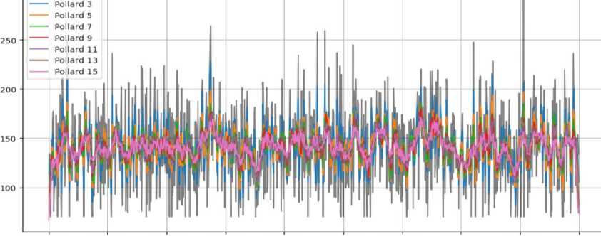
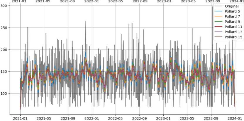
Fig.18. Pollard smoothing and Pollard resmoothing with increasing intervals

0	3	1000	0.S14144	0	5	1000	0.562712
1	5	1000 1000	0.694280 0.606710	1	7	1000	0.478329
2	7
3	9	1000	0.540404	2	9	1000	0.422553
4	11	1000	0.50261S	3	11	1000	0.389787
5	13	1000	0.473550	4	13	1000	0.367511
6	15	1000	0.445386	5	15	1000	0.343905

Fig.19. Table of smoothing results with intervals, turning points and correlation

The graphs in Fig. 21 demonstrate the autocorrelation functions for the original data (Original) and the smoothed series obtained by the Pollard method with different smoothing intervals (from 3 to 15). In the graph for the original data, a sharp decline in autocorrelation is observed already at the first lags, which indicates significant variability and shortterm dependence between the values. It shows a high level of noise in the original data. In the smoothed series (Pollard 3–15), the autocorrelation decreases more gradually. For small smoothing intervals (Pollard 3, 5), partial correlation is preserved at short lags, but it quickly decreases, which indicates effective smoothing of local fluctuations. In the series with larger smoothing intervals (Pollard 13, 15), the autocorrelation is preserved at longer lags, which indicates stronger smoothing and strengthening of long-term trends. Overall, these graphs show how smoothing affects the structure of the data, highlighting long-term trends. It can be useful for analysing data that requires identifying overall trends rather than short-term changes.

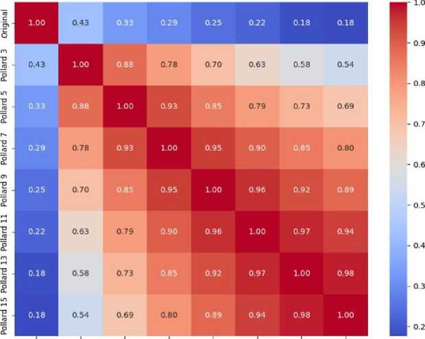
Original Pollard 3 Pollard 5 Pollard 7 Pollard 9 Pollard 11 Pollard 13 Pollard 15

Fig.20. Correlation matrix for smoothing

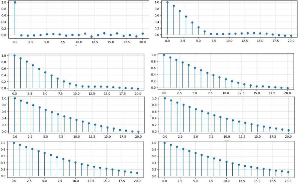
Fig.21. Autocorrelation for smoothing (left to right and top to bottom for Original, 3, 5, 7, 9, 11, 13, 15)

The graph in Fig. 22a shows the correlation field between blood glucose levels and body mass index (BMI). The points on the graph represent the relationship between two variables: glucose levels on the X-axis and BMI on the Y-axis. The distribution of the points appears chaotic, indicating a weak or absent relationship between these variables. The calculated Pearson correlation coefficient is 0.0232, which is very close to 0, indicating an almost non-linear relationship between glucose levels and BMI. The p-value is 0.4638, which is significantly higher than 0.05 and suggests that the correlation is not statistically significant. It means that the weak correlation found may be due to chance. In addition, the correlation ratio is 0.0070, confirming the low level of association between these indicators, even when nonlinear relationships are taken into account. Overall, the results of this analysis indicate that BMI and glucose levels do not have a significant relationship in the data under study. Either the two measures vary independently of each other, or their relationship is influenced by other hidden variables that are not included in this analysis.

The graph in Fig. 22b shows how blood glucose levels are related to themselves at different points in time. The x-axis shows the time intervals (lags), and the y-axis shows the degree of similarity between glucose values. As expected, at the beginning (lag 0), the correlation is 1.0 because the data are perfectly consistent with themselves. However, with each subsequent step, the correlation decreases rapidly and fluctuates around zero. It means that glucose levels do not show clear recurring trends or cycles over time. Simply put, glucose levels vary quite randomly and do not have a stable pattern that can be easily predicted based on previous data. This result suggests that more sophisticated analysis methods that take into account other factors than just time dependence may be needed to predict glucose levels.

The correlation matrix is in Fig. 23 for the three parts of the data. It shows weak correlations between the parts since the values are close to zero in most cases. For example, between the first and second parts, the coefficient is -0.0842, and between the first and third – 0.0092. It indicates that the series parts are almost unrelated. That is, the data in different segments behave independently. The multiple correlation coefficient (R²) is 0.0355, which indicates a very weak relationship between the parts. It means that the distribution of values does not have a clear structural dependence or typical pattern.

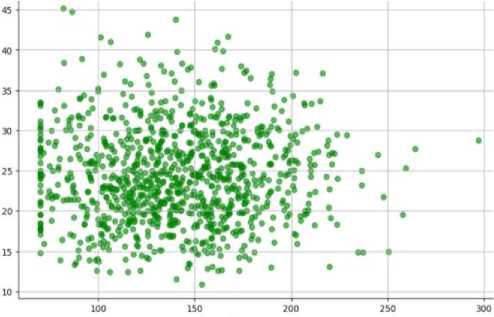
Fig.22. Correlation field between glucose level and BMI

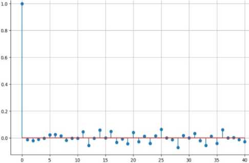
Parti

Part2

Part3

Parti

Part2

1.000000

-0.084198

-0.084198

0.009205

1.000000

-0.069319

and autocorrelation function for glucose level

Parti

0.009205

-0.069319

1.000000

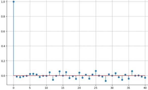
Fig.23. Autocorrelation function for the entire series

The graph in Fig. 23 shows the autocorrelation function for the entire series. The highest correlation is observed at the first lag (0.0), which is expected since the series is always maximally correlated with itself. However, with subsequent lags, the correlation drops sharply and fluctuates around zero. It once again confirms that the data do not have a noticeable periodicity or strong autocorrelation over long distances. The dendrogram in Fig. 24 displays the results of hierarchical cluster analysis, which uses Ward's clustering method to group objects based on their similarity. The vertical axis shows the distance or similarity measure between clusters, and the horizontal axis shows the objects being analysed. The colours of the lines indicate the selected groups (clusters) that were formed during the merging. The three main clusters are marked with different colours: orange, green, and red. They demonstrate how the objects gradually merged into groups, starting from the smallest distance and ending with large structures. The lower the merging of two elements, the closer they are to their characteristics. High mergers (blue lines) indicate less similar groups that merged in the last stages of the analysis. This plot is helpful in visualizing the hierarchy and choosing the optimal number of clusters. For example, it can be concluded that the three main clusters are sufficiently clearly separated, which can be confirmed by additional methods of clustering assessment.

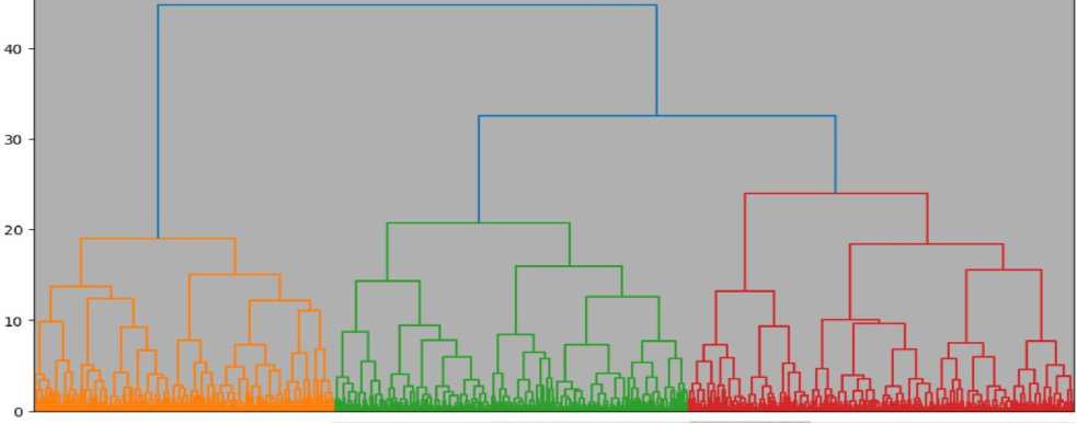
1 to 10 of 1000 entries | Fitter |D

___________0______________________t______________________г______________________3______________________4______________________5______________________В______________________Г______________________В______________________I

0.0                1.5122204380710004 1.020175608743031  4.004010830510721  2.7104090105322720 2.0877250334453908 2.7165844148035873 1.3343042605491078 3.3095073254212248 2.24119021

1.6122204309710894 0.0                2.7505474412020494 3.8070901430677744 3.2824380402317027 3.321402002204801  1.9800940494015204 2.7317582048057104 3.2807225664004007 2.1494941

1 820175500743031 2 7505474412020494 0.0                29096785413502473 1 7722153065358937 27810760574333857 27273443259702113 1 1447649006163658 25767312973537853 21933412'

4 064610639510721 38670981430577744 29898785413592473 0.0                3.3083350774335484 4.737371140134465  2.122466383737563  4019417535829240  3,17130939907376   2.9501074.

27104809105322726 3.2824366452317927 1.7722153065306937 3.3063350774335484 0.0                3.6030650153689917 3.326340532976561  2406340462622481  26112242517952953 34982581

26377256334453906 3.321462062264861  2.7810760574333657 4.737371140134465  36030650153689917 0.0                3.0731567350157935 2063494508246282  3.4010504768123175 3.0039317

2.7155844146635673 19806940494815204 2.7273448269792113 2.122460383787563  3.326840532976561  3.9731567350157935 0.0                33203353976083526 3.0874020810111757 1.84463871

1.3343042805491878 2.7317582848057184 1.1447649006108656 4.019417635829246  2.496340462822481  2.563494658246282  3.3203363976503526 0.0                3.310243902955204  2.48573051

33095073254212246 3.2607221564004667 2.5767312973537853 3.17130989907376   2.6112242517952953 3.4015504768123175 3.0874020619111757 3.310243902955204  0.0                2.5964302

2.241198282274707  2.1494941525141074 2.1933412583417846 2.9501074452894005 3.49825810544232   3.0039317174840923 1.8446387042872414 2.485730591608539  2.596436253001328  0.0

Fig.24. Hierarchical cluster analysis dendrogram and proximity matrix table

The proximity matrix table in Fig. 24 displays the distances between objects used for cluster analysis. Each row and column represent a separate object, and the numerical values in the table indicate the calculated Euclidean distance between pairs of objects. The values on the diagonal (from the upper left to the lower right) are zero since the distance of an object to itself is always zero. The smaller the value between two objects, the closer they are to each other in the multidimensional feature space. For example, objects 0 and 1 have a distance of 1.5122, while objects 0 and 8 have a greater distance of 3.3057, indicating less similarity between them. This matrix is the basis for constructing a dendrogram, where these distances are used to define clusters. Analysing such matrices helps to understand the structure of the data and identify groups of objects with similar characteristics.

The cluster analysis results table in Fig. 25a contains two columns: Object and Cluster. The Object column numbers all the objects in the data set, and the Cluster column indicates which cluster each object was assigned to base on the results of the hierarchical cluster analysis. For example, object 1 belongs to Cluster 5, object 2 to Cluster 2, and object 6 to Cluster 1.

Object		Cluster
1	5
2	2
3	5
4	3
5	5
6	1
7	3
8	5
9	5
10	3
11	5
12	2
13	2
14	2
15	5
16	3
17	1
18	5
19	2
20	1		Cluster
21	3		1    290
22	2		2    150
23	3		3    190
24	1		4    117
25	2		5    253

bloodglucose                             bmi                            physical_activity                        stress_level	hydration_level
■0.06634660344528932                -0.05087734184905156              -0.021168347362971872               0.018633364654103077	■1.5646967316604727
■0.040935333210349416               -0.2510612775821634               -0.6845974169047024                 1.1407759916011988	0.639101481945827
0.24156798626709078                0.28772977414542894               0.7197466671592664                 0.6794095240838164	0.639101481945827
0.29591930597303207                 1.106036627769695                 0.4703848745529949                 -0.9662983320670523	0.639101481945827
-0.21794332493638577                -0.520400481277219                -0.32789906645056804               -0.7610710640867577	0.639101481945827

Fig.25. Cluster analysis results table, cluster size table and cluster centre table

The table in Fig. 25b helps to identify groups of similar objects based on their characteristics. Clustering allows you to see the structure of the data and simplifies further analysis, for example, to identify patterns or features of each group. The results of this classification can also be used for further analysis, visualization or decision-making.

The cluster analysis results in Fig. 25b include cluster sizes and cluster centres. The table in Fig. 25 shows the cluster sizes, i.e. the number of objects included in each of the five clusters:

• •    Cluster 1 contains 290 objects.

• •    Cluster 2 contains 150 objects.

• •    Cluster 3 contains 190 objects.

• •    Cluster 4 contains 117 objects.

• •    Cluster 5 contains 253 objects.

It shows that the largest cluster is the first (290 objects), and the smallest is the fourth (117 objects).

The table in Fig. 24c presents the cluster centres, which display the average values of the normalized characteristics for each cluster for the following parameters:

• •    blood_glucose — blood glucose level.

• •    bmi — body mass index.

• •    physical_activity — physical activity level.

• •     stress_level — stress level.

• •    hydration_level — hydration level.

These values show the characteristics of each cluster. For example, some clusters may have higher levels of physical activity and lower levels of stress, while others may have the opposite. The results can be used to interpret behavioural or physiological groups in the sample, identify trends, and create profiles for different groups of subjects.

The graph in Fig. 26 shows the dependence of the mean value of the risk score on the level of stress. The x-axis indicates the stress levels, and the y-axis indicates the mean value of the risk. There is a tendency for the risk to increase with increasing stress levels. At zero stress levels, the mean risk score is the lowest, while at maximum stress levels, it reaches the highest value. These results indicate a positive relationship between stress and risk, which may indicate a higher vulnerability to adverse health outcomes among people with increased stress levels. The graph highlights the importance of further analysis of this relationship for the development of prevention measures.

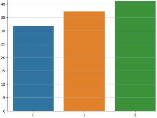
Fig.26. Average risk score for each stress level

This work conducted a comprehensive analysis of data related to the health and lifestyle of people with diabetes to identify patterns affecting blood glucose levels, BMI, physical activity, stress levels, and other parameters. The use of statistical methods, correlation, and cluster analysis allowed us to assess the relationships between indicators, identify significant trends and risk groups, and identify dependencies that may be useful for improving the diagnosis and treatment of diabetes. The use of smoothing methods, in particular the Kendall and Pollard formulas, made it possible to eliminate random fluctuations in the data and focus on the main trends. Smoothing with different intervals showed that short intervals are better suited for reflecting local changes, while longer intervals provide a more stable detection of long-term trends. Repeated smoothing with increasing intervals confirmed the effectiveness of combined approaches for trend analysis. The calculation of correlation coefficients and the number of turning points allowed us to assess the accuracy of the smoothed series in comparison with the original data. Correlation analysis showed a weak relationship between glucose levels and body mass index, which may indicate other, less obvious factors that influence glucose levels, such as stress levels, physical activity, and hydration.

The lack of strong correlations between these indicators emphasizes the need for a comprehensive approach to data analysis to identify latent patterns. Autocorrelation analysis showed that the data lacked clear cyclical patterns, which may indicate the difficulty of predicting short-term changes in glucose levels based on available parameters. Cluster analysis allowed us to divide the study subjects into groups based on the degree of similarity of their characteristics. The use of hierarchical clustering and the construction of a dendrogram revealed five main clusters that differ in the average values of glucose levels, BMI, physical activity and stress levels. It made it possible to identify groups with increased risks for further targeted research and the formation of recommendations. The proximal matrix obtained during the analysis demonstrated the distances between the subjects, confirming the internal similarity in each cluster. According to the results of cluster analysis, the largest groups are characterized by average values of glucose levels and BMI.

In contrast, smaller groups contain participants with extreme values of these parameters, which may indicate special health risks. Analysis of the average values of the risk indicator depending on the level of stress revealed a clear trend of its increase with increasing stress levels, which emphasizes the importance of managing stress factors for controlling the risks associated with diabetes. The results demonstrate the effectiveness of smoothing, correlation, and cluster analysis in exploring complex relationships in diabetes data. They also highlight the importance of combining different analysis methods to gain a deeper understanding of the impact of risk factors on glucose levels and the overall health of patients. The findings of this work can be used for further research and the development of personalized approaches to diabetes treatment and prevention.

5.    Results

Determining the distribution of diabetes incidence in the Pima Indians Diabetes dataset is a key step in the analysis and development of predictive models [45]. Illustrating this distribution through a bar chart and a percentage pie chart allows us to clearly display the relationship between the diseased and healthy individuals in the sample. The former (Fig. 27a) clearly shows the number of individuals diagnosed with diabetes compared to those who remain undiagnosed.

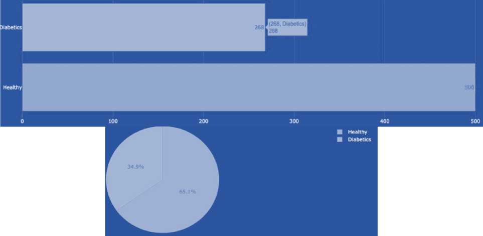
Fig.27. Number of healthy and sick people in the sample and percentage ratio of healthy and ill people

The pie chart (Fig. 27b), in turn, presents the same data in percentage terms, illustrating the proportion of diabetics out of the total number of respondents. It makes it possible to assess the relative proportionality of health conditions in the sample, which is especially useful when analysing the impact of morbidity on the population. The percentages in the pie chart are displayed clearly and clearly, providing easy access to information about the structure of the sample.

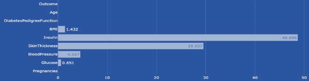
Fig.28. Percentage of missing data

Missing data in the Pima Indians Diabetes dataset can significantly impact the quality and validity of analytical findings because they create challenges for data processing and analysis. The problem of missing data arises for a variety of reasons, including errors in data collection, loss of records, or participants’ refusal to provide specific data. The presence of incomplete data requires the use of imputation methods, which may include the use of means, medians, or even more sophisticated statistical techniques, such as multiple imputation or modelling based on existing patterns in the data. These approaches allow for the recovery of missing information and provide greater accuracy and objectivity in the study results [46]. To visually demonstrate the extent of the missing data problem in the study, a chart that clearly shows the percentage of missing data for each metric in the dataset is planned to be created (Figure 28). It will help visually assess which variables are most frequently missing. It will contribute to a better understanding of the potential impact of these omissions on the study results, as well as on decisions about data entry and processing methods. In the Pima Indians Diabetes dataset, some key metrics have significant gaps, which may impact the quality of analytical results. The highest percentage of gaps is observed in insulin values (48.698%), a critical indicator for assessing diabetes status, followed by skinfold thickness (29.557%), body mass index (BMI) with gaps of 1.432%, blood pressure (4.557%), and glucose (0.651%). These gaps in the data require careful analysis and the correct choice of methods to ensure the accuracy and reliability of scientific conclusions.

A correlation matrix is a tool used to determine and display the degree of statistical relationship between different variables. The correlation between two values can range from -1 to 1, where 1 indicates a perfect direct correlation, -1 indicates a perfect inverse correlation, and 0 indicates no linear relationship. A high correlation between two variables means that when one variable changes, the other is likely to change in the predicted direction [47]. In the context of the Pima Indians Diabetes data, a high correlation can be found between measures such as glucose and insulin levels (0.58), indicating that higher blood glucose levels are often associated with higher insulin levels (Figure 29). There is also a high correlation between body mass index and skinfold thickness (0.65), highlighting the relationship between total body fat mass and fat deposits in specific areas. High correlation values in these cases may help identify the main factors influencing the development of diabetes and contribute to the development of more effective strategies for its prediction and management [48].

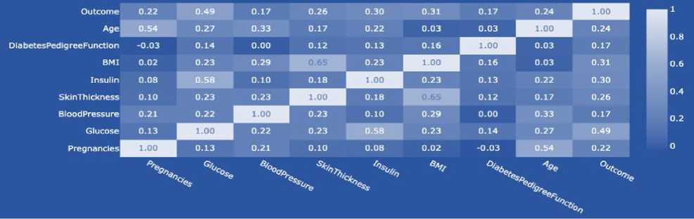
Fig 29. Correlation matrix for pima indians diabetes

Before proceeding to build a model, it is necessary to adequately prepare the dataset, in particular, fill in missing values. This process is essential because missing data can distort the results of the analysis and reduce the accuracy of the model. Using effective methods helps to restore lost information and ensure greater consistency and reliability of the data. In the context of the Pima Indians Diabetes dataset, insulin is a critical measure that reflects the level of insulin in the blood 2 hours after a glucose load. This measure is of great importance for assessing insulin resistance, which is often associated with type 2 diabetes. To better understand the impact of insulin on the health of individuals with and without diabetes, a graph was created that visualizes the distribution of insulin levels (Figure 30). In addition, median values for non-zero insulin measurements were determined, which were 102.5 for a healthy individual (0) and 169.5 for a person with diabetes (1). It confirms that insulin levels are higher in diabetic patients, which may indicate the presence of insulin resistance and the need for further medical intervention or monitoring. Analysis of the histogram of insulin levels in the dataset revealed that the distribution is right-skewed. This means that most of the values are concentrated above the median, and there is a long tail of lower values that extends to the left. A left-skewed distribution often indicates that lower insulin values are more common, but there are also rare cases with significantly higher levels (Figure 31a). In cases where the data distribution is skewed, imputation of missing data using the mean may not be the best solution, as outliers may bias it. Instead, using the median to impute missing values is more appropriate, as the median is robust to outliers and better reflects the “central” value in the case of skewed distributions.

Glucose plays a key role as it is the leading indicator used to diagnose diabetes. The blood glucose level after an overnight fast is an important indicator. High glucose levels may indicate a disruption in this process, which is typical of diabetes (Fig. 32). Analysis of glucose levels, similar to insulin analysis, includes studying its distribution among the study participants. Median glucose levels were 107 for healthy individuals (0) and 140 for individuals with diabetes (1). These data confirm that individuals with diabetes have higher baseline glucose levels, which is indicative of metabolic abnormalities associated with the disease [49]. An essential aspect of the analysis is also determining the shape of the glucose distribution. In this case, we have the glucose distribution not to have a pronounced asymmetry (Fig. 31b), which indicates a more uniform distribution of values. In such conditions, using the mean value to fill in the missing data is appropriate since the mean provides an accurate estimate of the central tendency of the distribution without the bias that could arise due to asymmetry [50]. Thus, the mean is used to enter missing glucose values, which ensures the preservation of the internal structure of the data and contributes to the accuracy of subsequent analyses and modelling.

Triceps skinfold thickness is one of the anthropometric measures used to assess the level of subcutaneous fat in the body. This measure is essential because it may indicate an increased risk of developing insulin resistance and type 2 diabetes, especially if it is above the norm (Fig. 33). In the Pima Indians Diabetes data set, the median values of triceps skinfold thickness are 27 mm for healthy individuals (0) and 32 mm for individuals with diabetes (1), reflecting a general trend towards higher values in the diabetic group. Analysis of the distribution of this measure showed that the data are right-skewed. That is, most of the values are concentrated at the low end of the scale, but there are a significant number of high values that pull the mean towards higher numbers (Fig. 34a). In this regard, the use of the median was chosen to fill in the missing values.

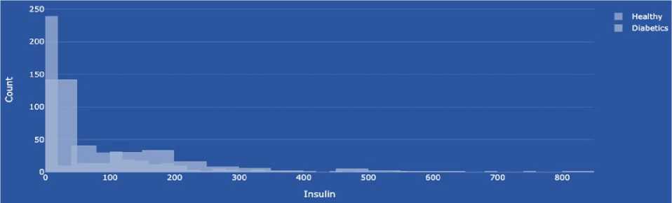
Fig.30. Distribution of healthy and sick people depending on insulin levels

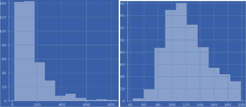
Fig.31. Histogram of insulin and glucose levels

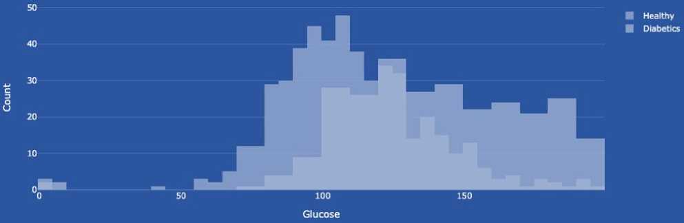
Fig.32. Distribution depending on glucose level

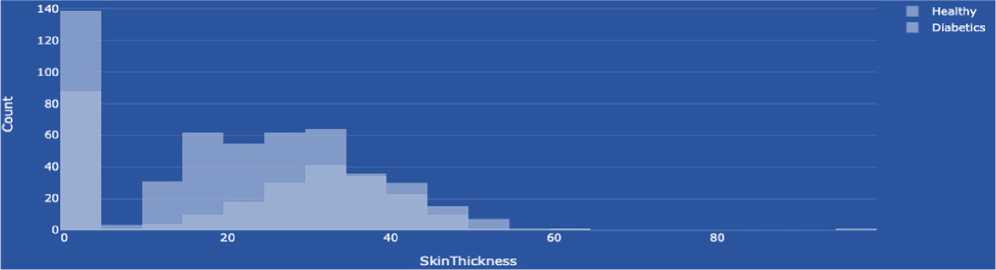
Fig.33. Distribution of triceps skinfold thickness values

Blood pressure in the context of the Pima Indians Diabetes dataset plays a significant role, as high blood pressure is one of the risk factors for developing type 2 diabetes and its complications (Fig. 35). In this study, the analysis of blood pressure levels showed that the mean values are 70 mm Hg for healthy individuals (0) and 74.5 mm Hg for individuals with diabetes (1), indicating a slightly higher pressure in the diabetic group. It was found that they do not have an apparent asymmetry to determine the distribution of blood pressure in the analysed data. It means that the data are distributed more or less evenly around the mean value, without pronounced tails of high or low values (Fig. 34b). Therefore, the mean value is used to fill in the missing data, as it accurately reflects the central tendency in the case of a normal distribution, ensuring objectivity and accuracy in the recovery of missing values.

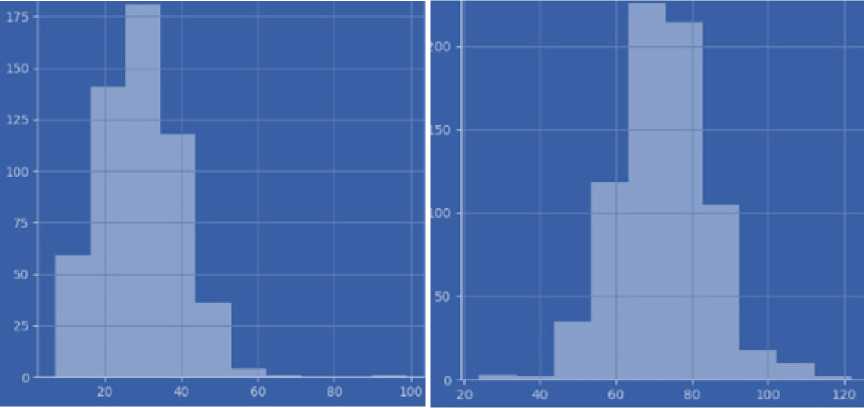
Fig.34. Histogram of triceps skinfold thickness and distribution of blood pressure values

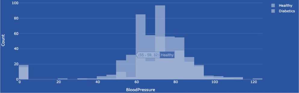
Fig.35. Blood pressure distribution

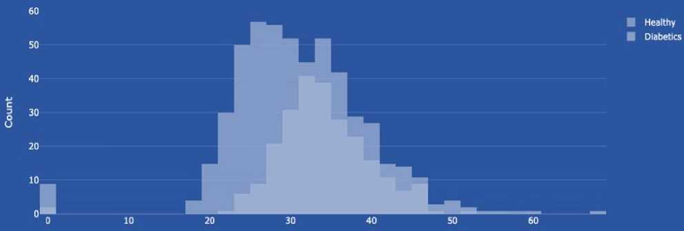
Fig.36. Distribution of body mass index values

Body mass index (BMI) is an essential indicator in the context of research, as it helps to assess a person's physical condition and the risk of developing diabetes (Figure 36). BMI is calculated as the ratio of body weight (in kilograms) to the square of height (in meters). BMI values can be used to determine whether a person is in the normal weight range, underweight, overweight, or obese. To assess the risk of developing diabetes, it is essential to pay attention to overweight and obesity, as these conditions significantly increase the risk of insulin resistance and, as a result, the development of type 2 diabetes. In this study, the mean BMI values were 30.1 for healthy individuals (0) and 34.3 for individuals with diabetes (1), which confirms the relationship between higher BMI values and the presence of diabetes. The distribution of BMI in the dataset is skewed, with a bias towards higher values. It indicates that the study group contains individuals with high BMI, which can significantly affect the mean value (Fig. 37). Therefore, to correctly fill in the missing data, it was decided to use the median, which better reflects the typical BMI value for this sample and provides greater accuracy of the analysis without the bias that extreme values could cause.

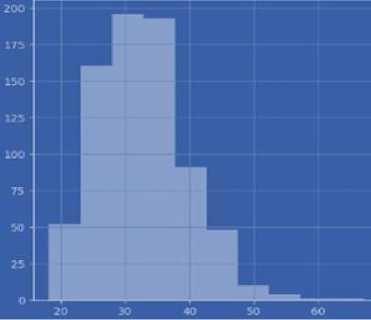
Fig.37. Distribution of body mass index values

After filling in the missing values, it is essential to perform a data completeness check to ensure that the data is complete and ready for further analysis and modelling. This step is critical because it allows us to confirm that all expected datasets have been adequately processed and that there are no more gaps in the data that could affect the results of the work [50]. After a thorough inspection of the data, it was determined that there were no gaps in the dataset (Fig. 38a).

Outcome *9*
D'abet es₽edio гее ► unction BMI Insulin Sk*nTb*ckn##o Blood Pressure Glucose Pregnancies -1 ЙЗ tr           S raws * : Z Pregnancies * I		5 raws x 8 columns 2 Glucose : 1	-0 5 BloodPressure : 2	SkinThickness :	0 2 Insulin :	BMI :	O.5 я DiabetesPedigreeFunction     :		1 ± I? @ 1 Age :
9	0,639947	0,865108	-0.033518	0.670643	-0.181541	0.166619		0.468492	1.425995
1	'0.844885	•1.296162	•0.529859	•0.012381	-0.181541	-0.852200		-0.365061	-0.190672
2	1.233880	2.015813	-0.695306	-9.012301	-0.181541	-1.332500		0.604397	-0.105584
3	-0.844885	-1,074652	-0.529859	-0,695245	-0,540642	-0.633881		-6.920763	-1.041549
4	-1.141852	0.503458	-2.680669	0.670643	0.316566	1.5493G3		5.484909	-0.020496

Fig.38. Checking for missing values after filling them in

Data scaling is a critical step before training machine learning models (Figure 38b), especially when using the k-nearest neighbours (k-NN) algorithm. Scaling is due to the fact that k-NN determines the similarity between cases based on their distances in a multidimensional space, and the presence of attributes with different scales can lead to distances being dominated by those attributes that have higher absolute ranges of values:

• •    uniform influence, i.e. without scaling, attributes with large value ranges can disproportionately influence the determination of distances between cases, which can lead to distortion of classification results. For example, an attribute with a range from 0 to 1000 will affect the distance much more than an attribute with a range from 0 to 1;

• •    improving accuracy, for example, scaling helps to ensure that each attribute contributes equally to the determination of similarity between cases. It contributes to a more accurate and fair calculation of distances, especially in algorithms that are sensitive to the scale of attributes;

• •    increasing the speed of learning, in particular, scaling, can also help speed up learning processes since optimization algorithms often work more efficiently when the data is at the same scale. It reduces the risk of getting stuck in local minima and contributes to better algorithm convergence.

Splitting data into training and test sets is a fundamental step in the machine learning process, as it allows us to evaluate the quality and performance of a model in conditions that are close to real-world use [51]. The train_test_split function from the sklearn library helps us to implement this split by assigning a part of the data to train the model and the rest to validate it. In this case, the data is split so that one-third is used for testing and the rest for training. The use of the random_state parameter ensures reproducibility of the results by fixing the initial state of the random number generator, and stratify=y ensures that the original class proportions represented by the variable y are preserved in the training and test sets. Initially, an experiment was conducted with different numbers of neighbours (from 1 to 19) to find the optimal value for k-NN. As a result of the analysis of the “Train and Test Score with neighbours” graph, the best value of the parameter k was found to be 11, as this value provided the highest balance between accuracy on the training and test data sets (Fig. 39a). After training the k-NN model using 11 neighbours, the model’s performance was evaluated using several key metrics:

• •    the confusion matrix showed that 142 cases were correctly classified as healthy and 54 cases as sick, indicating a relatively high ability of the model to distinguish between states (Fig. 39b);

• •    the classification report indicated an accuracy of 0.77 with a fixed accuracy of 0.80 for healthy and 0.68 for sick, with corresponding recall indicators (Fig. 40a);

• •    the ROC curve and AUC score showed a high ability of the model to distinguish between classes, with an AUC score of 0.819, indicating a fairly high overall efficiency of the model in the conditions of classification tasks (Fig. 40b).

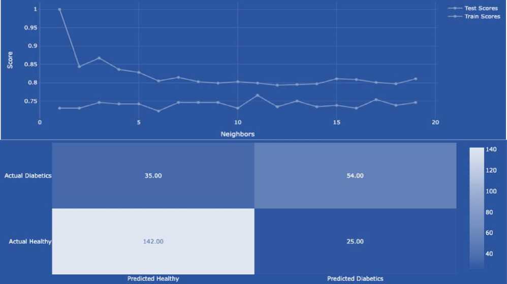
Fig.39. "Train and test score with neighbours’ graph and confusion matrix

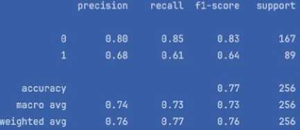
Fig.40. Classification report and ROC curve

Hyperparameter optimization is a key aspect of building effective machine-learning models. This process allows you to tune the model so that it achieves the best possible performance. For k-nearest neighbours (k-NN), the main tunable hyperparameter is n_neighbors , which is the number of neighbours that directly affects the classification results. After optimization, the results showed that the best model performance was achieved at n_neighbors = 25 with an accuracy of approximately 0.772. It indicates that the model with this parameter optimally balanced between a small and a large number of neighbours, providing the best generalization. Hyperparameter optimization via GridSearchCV has been beneficial for improving the k-NN model by identifying the value that provides the best overall performance. This process is an essential step in preparing the model for real-world applications, as it allows you to adapt the model to specific usage conditions and tasks [51-52]. The knowledge gained can be used for further research and development in the field of diabetes prediction, as well as to improve medical strategies based on data analysis.

We will describe the process of selecting the optimal value к (number of neighbours) when optimising the hyperparameter for the k-NN model, which is vital for ensuring scientific transparency and reproducibility of the results.

To improve the quality of forecasting and prevent overtraining, parametric optimisation of the hyperparameters of the k-nearest neighbour (k-NN) model was carried out, in particular the parameter n_neighbors, which determines the number of neighbours taken into account when classifying a new sample.

A setup strategy in the form of brute-force is used, i.e. Grid Search to select the optimal value к in a given range, using k-fold cross-validation.

• •    – Tool: GridSearchCV from the scikit-learn library;

• •    - Range of checked values к : from 1 to 20;

• •    – Optimisation criterion: maximisation of average accuracy on validation sets;

• •    - Number of folds: 5 (i.e. cv = 5 );

• •    – Data standardisation: performed preliminarily before cross-validation.

Implementation in Python:

from sklearn.neighbors import KNeighborsClassifier from sklearn.model_selection import GridSearchCV from sklearn.preprocessing import StandardScaler scaler = StandardScaler()# Scaling features

X_scaled = scaler.fit_transform(X)

best_k = grid_search.best_params_['n_neighbors'] # Best parameter value best_score = grid_search.best_score_

In the course of the search, the best value of the hyperparameter n_neighbors turned out to be к = X (where X — substitute the actual value from the study, for example к = 7 ), which provided average accuracy Y% on validation sets.

We will describe the use of cross-validation or any other data partitioning technique to reliably estimate the performance of the model. It is an essential stage of the study, since a single breakdown into training and test samples can lead to an overestimation or underestimation of the effectiveness of the model.

Validation is the process of evaluating the performance of a model not only on the data on which it was trained, but also on independent subsets to test its ability to generalise to new data.

• •    The principle of K-fold Cross-Validation (k-fold cross-validation) is that the data is divided into k equal parts (folds). The model is trained on k-1 parts and tested on the remaining one. The process is repeated k times. Each part is used once as a test part. The results are averaged. This process provides a robust performance assessment and reduces reliance on random data sharing. Example:

from sklearn.model_selection import cross_val_score from sklearn.ensemble import RandomForestClassifier scores = cross_val_score(RandomForestClassifier(), X, y, cv=5)

• •    Stratified K-fold Cross-Validation is the same as k-fold, but retains the proportions of classes (e.g. 65% healthy and 35% sick) in each fold. There is an imbalance of classes in the Pima Indians Diabetes dataset so that random splitting can lead to skew — for example, 90% healthy in the test set.

from sklearn.model_selection import StratifiedKFold skf = StratifiedKFold(n_splits=5)

X_train, X_test = X[train_index], X[test_index]

• •    Leave-One-Out Cross-Validation (LOOCV) is an extreme variant of k-fold, where k = N (number of examples). This validation is very accurate, but computationally expensive.

• •    Train/Test Split is the simplest but unreliable method. It can give skewed results, especially with class imbalances or small samples.

from sklearn.model_selection import train_test_split

X_train, X_test, y_train, y_test = train_test_split(X, y, test_size=0.2, stratify=y)

In medical tasks such as diabetes prediction, the generalizability of the model is a key requirement. Without proper validation, there is no certainty that the results are stable and that the risk of missing patients (FN) can be misestimated. The results are difficult to replicate or compare with other studies.

To ensure robust and generalisable model performance, stratified k-fold cross-validation should be employed, especially in datasets with imbalanced classes such as the Pima Indians Diabetes dataset. This method maintains the class distribution across all folds and provides a more reliable estimate of the model's actual predictive capacity. Future iterations of the system could benefit from using 5-fold or 10-fold stratified validation to assess the stability of results across diverse subsets of patient data.

A one-time validation by dividing into training and test samples using the train_test_split function from the sklearn library is implemented. The distribution was made in such a way that one-third of the data was used as a test sample, while the stratify=y parameter was applied to preserve the proportion of classes. The advantage lies in maintaining a balance between classes in the samples (necessary in case of imbalance). The disadvantage is that this approach provides only one estimate of efficiency, which may depend on a specific random division. After breaking down and training the k-NN model with optimal k=11, accuracy ~0.77, accuracy for class "healthy" 0.80, accuracy for class "sick" 0.68, ROC-AUC is 0.819. In the confusion matrix, 142 "healthy" and 54 "sick" are classified correctly.

It is desirable to supplement cross-validation with stratified k-fold cross-validation, which takes into account the class imbalance with each split. It gives an average value of metrics, which makes the assessment more reliable. For example, StratifiedKFold(n_splits=5) provides training/testing on five different subsets and averaging metrics (Accuracy, F1-score, ROC-AUC, etc.).

from sklearn.model_selection import StratifiedKFold, cross_val_score from sklearn.neighbors import KNeighborsClassifier skf = StratifiedKFold(n_splits=5)

model = KNeighborsClassifier(n_neighbors=11)

scores = cross_val_score(model, X, y, cv=skf, scoring='roc_auc')

In the current study, the evaluation of the effectiveness of the model was carried out by a single breakdown into training and test samples using the train_test_split function with the stratify=y parameter, which allows you to preserve the proportions of the classes. This approach provides a basic quality check of the model, but the results may depend on the specific division of the data. To increase the reliability and generalizability of forecasts, it is advisable to use crossvalidation, in particular, Stratified k-fold cross-validation. This approach allows the model to be repeatedly trained and tested on different subsets of the data, while maintaining the class ratios in each sample. Averaging the results obtained will enable you to get a more objective assessment of the quality of the model. Especially in the face of class imbalances inherent in the Pima Indians Diabetes dataset, the use of stratified cross-validation helps to avoid sample bias and reduce the risk of overlearning. In further stages of the study, it is advisable to implement this method of evaluation in order to increase the reliability of the results obtained and make the conclusions more reasonable from a practical point of view.

Although the current evaluation relies on a one-time train-test split with stratification, further validation using stratified k-fold cross-validation is recommended. This approach ensures more reliable and generalisable estimates of model performance by testing the model on multiple data subsets. Especially in medical datasets with class imbalance, such as the Pima Indians Diabetes dataset, stratified validation helps maintain consistent class proportions. It avoids overfitting to a single partition of the data.

6.    Discussion

Data Analysis to Predict the Development of Diabetes

In the realm of blood glucose analysis, it is essential to recognize the existence of various diabetes subtypes, as well as conditions indicating a predisposition to the disease. Recalling the definition, diabetes is a chronic condition that impacts the body’s ability to transform food into usable energy. Typically, carbohydrates from food are broken down into glucose, which enters the bloodstream. A rise in blood glucose triggers the pancreas to release insulin, a hormone that enables glucose to enter cells and provide energy. However, in individuals with diabetes, this process is disrupted – either the body does not produce sufficient insulin, or it cannot use the insulin effectively. As a result, glucose remains in the bloodstream at elevated levels. Persistent high blood sugar can lead to severe complications over time, including cardiovascular disease, vision impairment, and kidney damage. There are three main types of diabetes, but in the scope of open-source medical data, the focus is primarily on type 2 diabetes.

Additionally, diabetes mellitus is often classified into two stages: Prediabetes, which indicates elevated blood sugar levels not yet high enough to be diagnosed as diabetes, and Diabetes mellitus, the full onset of the disease. The work will build a model for predicting diabetes in patients. First, we will analyse the data on the basis of which research and the construction of a model and algorithm for predicting the incidence of type 2 diabetes will be conducted. The data set “diabetes _ 012 _ health _ indicators _ BRFSS2015.csv” containing 253,680 responses, was used as input data. The target variable includes three classes:

• – 0 – for people who do not have elevated blood glucose levels;

  – 1 – for people who are prone to diabetes (prediabetic state); – 2 – for people with diabetes.

# Diabetes.... ="	# HighBP		# HighChol		# CholCheck ="	# BMI		# Smoker		# Stroke
0 0	1.0		1.0		1.0	40.0		1.0		0.0
0.0	0.0		0.0		0.0	25.0		1.0		0.0
0.0	1 .0		1.0		1.0	28.0		0.0		0.0
0.0	1 .0		0.0		1.0	27.0		0.0		0.0
0.0	1.0		1.0		1.0	24.0		0.0		0.0
0 0	1.0		1.0		1.0	25.0		1.0		0.0
0.0	1 .0		0.0		1.0	30.0		1 .0		0.0
Diabetes.Ol 2	HighBP HighChol		CholCheck	BMI	Smoker Stroke	HeartDiseaseorAttack		PhysActivity	Fruits ... A
0  0.0	1.0       1.0		1.0	40.0	1.0       0.0	0.0		0.0	0.0	...     1
1   0.0	0.0      0.0		0.0	25.0	1.0       0.0	0.0		1.0	0.0	...    0
2  0.0	1.0       1.0		1.0	28.0	0.0      0.0	0.0		0.0	1.0	...     1
3  0.0	1.0      0.0		1.0	27.0	0.0      0.0	0.0		1.0	1.0	... 1
4  0.0	1.0       1.0		1.0	24.0	0.0      0.0	0.0		1.0	1.0	... 1

Fig.41. Part of the data for predicting the development of diabetes and presenting the characteristics in a table

The data reflect 21 characteristics that affect the development of diabetes, and the data themselves are unbalanced. That is, the number of people belonging to different classes is different. A fragment of the dataset is shown in Fig. 41a. To build a model for predicting the development of diabetes, it is proposed to use the Python programming language and a set of open machine-learning libraries. Next, it is necessary to display the factors that influence the development of diabetes and are present in the data set. As a result, we will obtain a result that shows the structure of the data set in the form of a table (Fig. 42) and the type of characteristics of individuals regarding their susceptibility to diabetes (Fig. 41b).

Rangeindex: 253680 entries, 0 to 253679 Data columns (total 22 columns): #   Column                Non-Null Count   Dtype 0   Di.abetes_012          253680 non-null  float64 1   HighBP                253680 non-null  float64 2   HighChol              253680 non-null  float64 3   CholCheck             253680 non-null  float64 4   BMI                   253680 non-null  float64 5   Smoker                253680 non-null  float64 6   Stroke                253680 non-null  float64 7   HeartDiseaseorAttack 253680 non-null  float64 8   PhysActivity          253680 non-null  float64 9   Fruits                253680 non-null  float64 10  Veggies               253680 non-null  float64 11  HvyAlcoholConsump     253680 non-null  float64 12  AnyHealthcare         253680 non-null  float64 13  NoDocbcCost           253680 non-null  float64 14  GenHlth               253680 non-null  float64 15  MentHlth              253680 non-null  float64 16  PhysHlth              253680 non-null  float64 17  DiffWalk              253680 non-null  float64 18  Sex                   253680 non-null  float64 19  Age                   253680 non-null  float64 20  Education             253680 non-null  float64 21  Income                253680 non-null  float64 dtypes: float64(22) unique value count Diabetes_0!2 3 HighBP 2 HighChol 2 CholCheck 2 BMI 84 Smoker 2 Stroke 2 HeartDiseaseorAttack 2 PhysActivity 2 Fruits 2 Veggies 2 HvyAlcoholConsump 2 AnyHealthcare 2 NoDocbcCost 2 GenHlth S MentHlth 31 PhysHlth 31 DiffWalk 2 Sex 2 Age 13 Education 6 memory usage: 42.6 MB

Income               3

Fig.42. Types of characteristics of people and their susceptibility to diabetes and the number of unique records in the data set

The following characteristics that influence the development of diabetes mellitus in this data set are identified: high blood pressure; high cholesterol; use of drugs to normalize cholesterol levels; body mass index; smoking; stroke; heart attacks; physical activity; consumption of vegetables; consumption of fruits; consumption of alcohol; any health care measures; general physical health; general mental health; sports walking; age; gender; education; income, etc.

A heat map is proposed to establish the correlation between the characteristics of the data set. The result of the correlation analysis is presented in Fig. 43. After data transformation, the number of unique records for each column of the data set was obtained, which interprets each characteristic. The distribution of data in the data set by categories 0, 1, and 2 is shown in Fig. 44. As can be seen from Fig. 44a, the data is very unbalanced, so balancing measures must be taken. It will allow in the future to build effective prediction models and identify factors that most affect the development of diabetes. To determine the correlation between factors that affect the development of diabetes, it is necessary to programmatically implement visualization of the dependence of blood sugar levels on the characteristics available in the data set. Fig. 45 shows the dependence implemented by the program code.

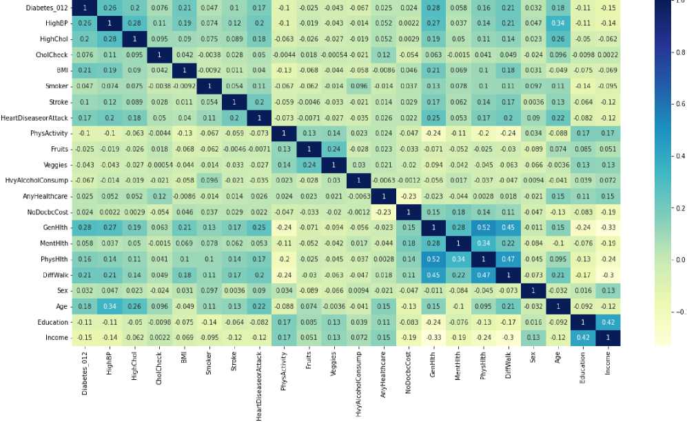
Fig 43. Correlations between data in a dataset

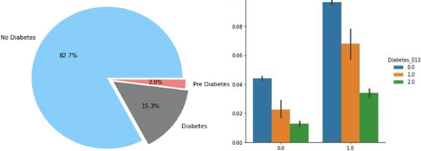
Fig.44. Distribution of data by target variable and dependence of diabetes development on smoking and alcohol consumption

Next, a visual analysis of the graphs was carried out on the influence of individual factors that affect the development of diabetes. So, in Fig. 46, as examples, the distribution of patients by gender and those who smoke and do not smoke is given. Analysing the histogram of Fig. 46, we can say that among the available data, more male individuals do not have diabetes. Among patients with elevated glucose levels, there are slightly fewer women, and the prediabetic state is also almost evenly distributed between women and men.

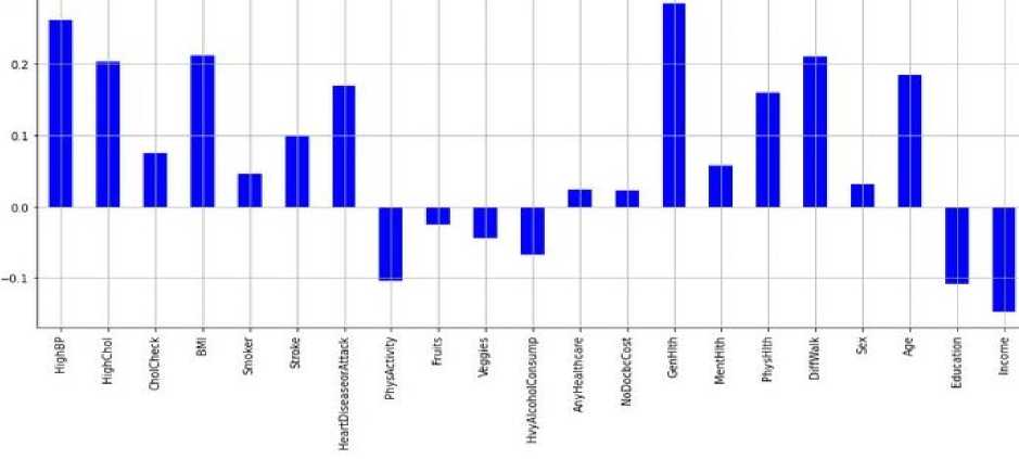
Fig.45. Correlation between factors influencing the development of diabetes and blood sugar levels

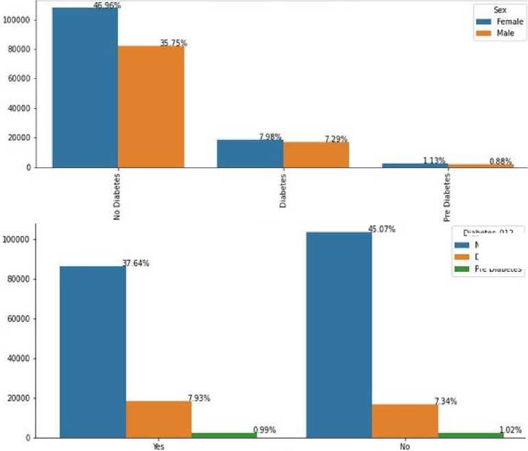
Fig.46. Distribution of diabetes incidence data by gender

Diabetes. 012 No Diabetes Diabetes Pre Diabetes

As can be seen from Fig. 46, the percentage of people who do not smoke is higher than the percentage of those who do not smoke. However, the presence of signs of diabetes is practically the same for both groups. After analyzing each of the twenty-one characteristics of the data set and their combinations, it was found that there is a dependence on the development of diabetes for groups of people who drink alcohol and smoke. Fig. 44b shows this influence graphically. As a conclusion from Fig. 44b - alcohol and smoking contribute to the development of prediabetes.

High cholesterol and high blood pressure are closely related (Figure 45a), as people with high cholesterol tend to have high blood pressure. The relationship between high blood pressure and high cholesterol goes both ways. When the body cannot remove cholesterol from the blood, excess cholesterol can build up on the walls of the arteries. When the arteries become stiff and narrowed by deposits, the heart has to work overtime to pump blood through them. It leads to high blood pressure.

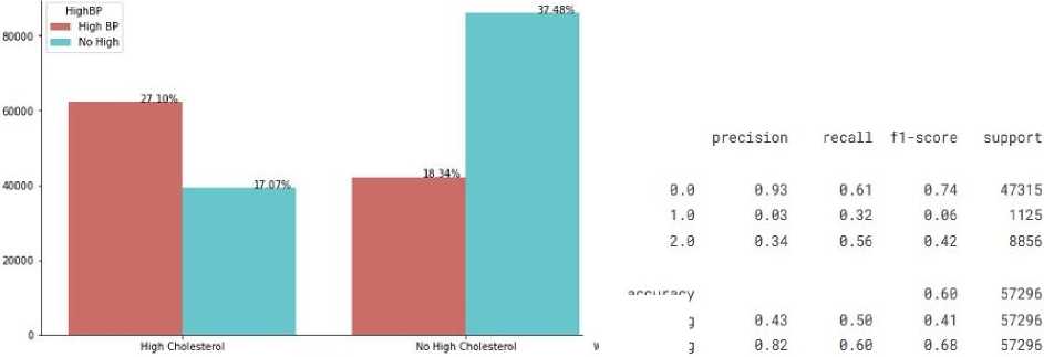
accuracy macro avg weighted avg

Fig.47. Dependence of blood glucose level on cholesterol level and assessment of the quality of the logistic regression algorithm

After conducting a preliminary analysis of the data available in the data set, it is necessary to perform a more detailed pre-processing of them. Data pre-processing should begin with the detection of outliers. To do this, first, you need to visually verify their presence. The program code allows you to generate the graph presented in Fig. 46a for outlier analysis. As can be seen from Fig. 46a, the obvious outliers of the data set are the values by the body mass index (BMI) attribute. However, in order to verify the truth of this assumption, it is necessary to visualize the values by all characteristics in more detail (Fig. 46b). Finding specific outlier values by the attribute of excess body weight involves executing the program code. If we visually present the values by BMI, then the distribution by value >70 and ≤ 70 will look like shown in Fig. 47. After performing such manipulations, it is necessary to remove the data that are outliers and recreate the data set. Having an updated data set is required to proceed to modelling algorithms for predicting the development of diabetes and determining the most critical factors that influence it.

The following conclusion can be drawn summarizing the analysis of visual information on the correlation of factors influencing the development of diabetes:

• •    men and women are equally vulnerable to diabetes;

• •    people over 45 years old are more susceptible to diabetes than younger people;

• •    the number of diabetics also increases with age;

• •    more than half of diabetics are obese, almost half of prediabetics are obese, and the percentage of diabetics and prediabetics who are obese and overweight is much higher than the percentage of non-diabetics who are obese and overweight – when education increases, the number of people with diabetes decreases;

• •    people with lower incomes have a higher risk of developing diabetes than people with higher incomes;

• •    genetics have a significant influence on diabetes. That is, when genetic indicators are bad – the risk of diabetes increases rapidly;

• •    mental (psychological) is the main factor that causes diabetes and depends on its stability over a long period;

• •    physical activity reduces the risk of diabetes;

• •    eating at least one fruit per day reduces the risk of diabetes;

• •    eating at least one vegetable per day also reduces the risk of diabetes.

It should be noted that when predicting blood sugar levels, it is necessary to solve the classification problem and determine the set and priority of factors that most affect the development of diabetes. In this case, forecasting is interpreted as prediction and not forecasting the development of diabetes over time – forecast. As noted earlier, forecasting the development of diabetes will be solved using classification methods. From a practical point of view, the most effective algorithms for solving a problem of this class are logistic regression, decision trees, XGBoost, and random forest. Logistic regression, as well as simple linear regression, were borrowed from the section on mathematical statistics. A distinctive feature of logistic regression is that a probability represents the value of the function.

Logistic regression, in principle, like linear regression, takes one or more independent variables as input and calculates the effect or dependence on the target variable. The difference between logistic and linear regression is the use of a sigmoid function, which makes it possible to predict a continuous variable in the range from 0 to 1 for any values of the independent variables. In fact, logistic regression is a Bernoulli distribution. The assessment of the criteria for prediction accuracy using the logistic regression approach is shown in Fig. 45b. The implementation of the prediction accuracy assessment using the ROC-AUC curve is about 73%. The error matrix shows the correspondence in terms of the number of correctly predicted values. It is shown in Fig. 48a. The following algorithm for predicting the development of diabetes mellitus is to implement the random forest approach. The quality of the classification results when executing the code is shown in Fig. 48b.

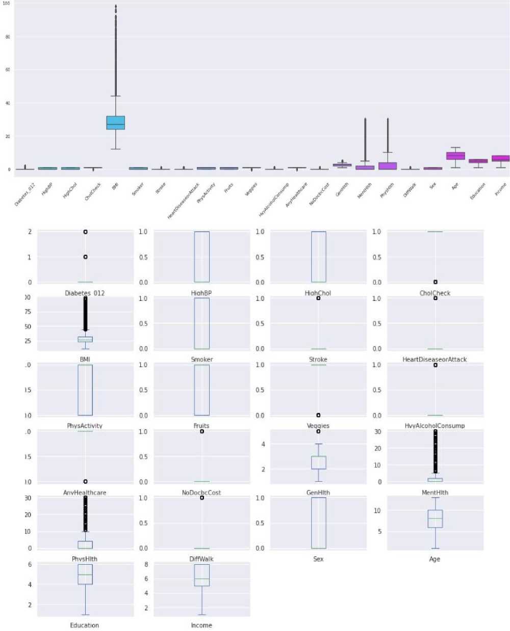
Fig.48. Visual representation of outliers and scatter of values for all attributes of the data set in the study of the development of diabetes mellitus

The value of the prediction accuracy assessment using the ROC AUC metric is about 75% and is illustrated in Fig. 49a. When evaluating the performance of the XGBoost algorithm, classification accuracy was achieved on various metrics at a level of 85% to 92%, which is shown in Fig. 49b.

The value of the ROC AUC metric when using the XGBoost algorithm is about 73% and is illustrated in Fig. 50. Another algorithm that can provide high accuracy in predicting the development of diabetes is decision trees. The results of the quality of the decision tree classifier are shown in Fig. 50b.

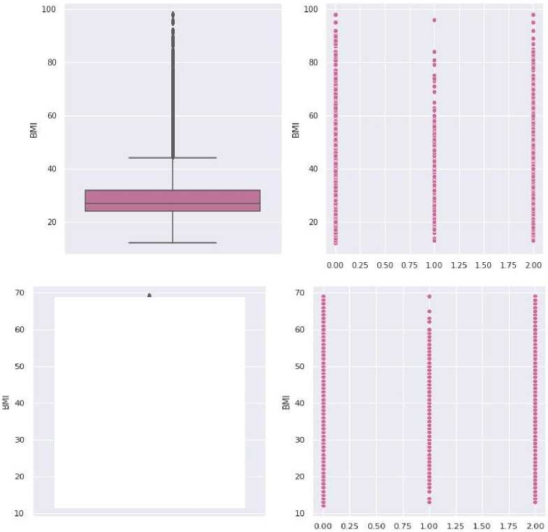
Fig.49. Detection of emissions based on body mass index

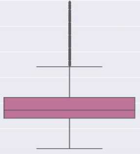
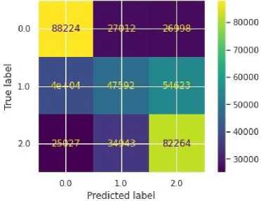
precision

0.00.87

1.00.06

2.00.44

accuracy macro avg0.46

weighted avg0.79

recall	f1-score	support
0.91	0.89	47315
0.00	0.01	1125
0.38	0.41	8856
	0.81	57296
0.43	0.44	57296
0.81	0.80	57296

Fig.50. Error matrix in predicting diabetes development and assessing the quality of classification results using the random forest approach

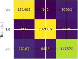
-120000

o.o 10          2.0

Predicted label

100000 - 80000 precision - 60000 0.0       0.85 1.0       0.20 - 40000 2.0       0.49 - 20000 accuracy macro avg       0.51 weighted avg 0.78

recall	fl-score	support
0.96	0.90	47315
0.00	0.00	1125
0.22	0.30	8856
	0.83	57296
0.39	0.40	57296
0.83	0.79	57296

Fig.51. Prediction evaluation using the ROC AUC metric and evaluation results of the XGBoost algorithm

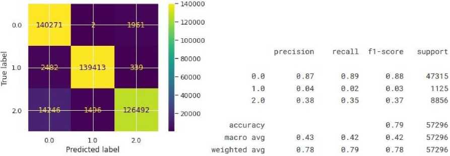
Fig.52. Estimation of prediction accuracy using ROC AUC and prediction quality results using decision trees

The quality assessment using the ROC AUC metric of the decision tree algorithm is approximately 70%. The result of comparing the quality of algorithms in predicting the development of diabetes is shown in Fig. 51. To increase the prediction accuracy, it is necessary to determine the most critical factors influencing the growth of diabetes. For this, appropriate manipulations were implemented, and a list of the essential signs of diabetes development was ranked (Fig. 52).

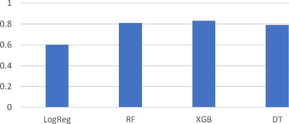
Fig.53. Evaluating the effectiveness of algorithms

After conducting repeated modelling based on 14 features with the most significant impact on the development of diabetes, the results of prediction accuracy at the level of 99% were achieved. Summarizing the results of the modelling, the following results were obtained:

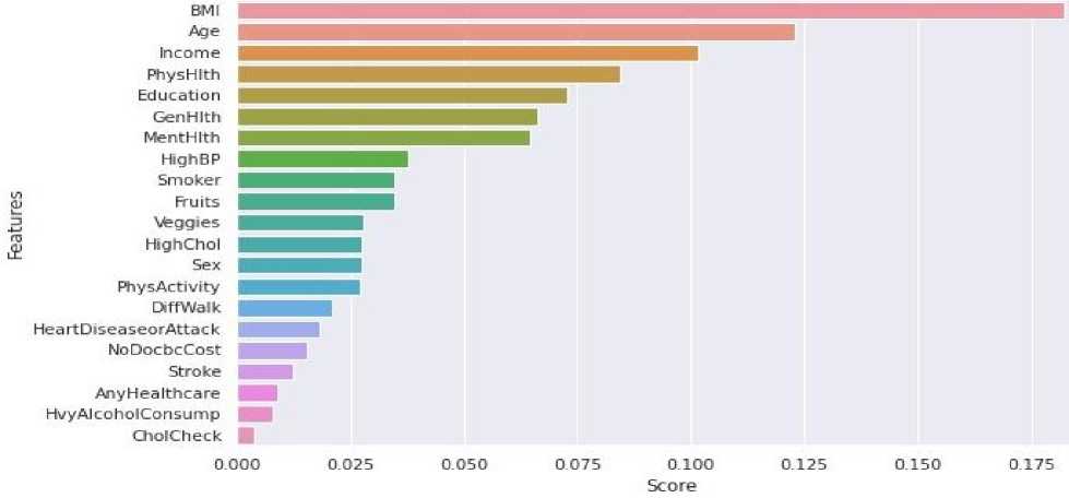
Fig.54. The importance of signs in influencing the development of diabetes

• •    The main features of diabetes are high blood pressure, high cholesterol, body mass index, stroke, general level, mental level, physical level, age, education and income.

• •    Characteristics that, in combination, increase the risk of diabetes are smoking and excessive alcohol consumption, stroke and cardiovascular diseases or heart attacks, and high blood pressure and cholesterol levels.

• •    Functional variables that have the least influence on the development of diabetes but can help reduce this risk are physical activity, consumption of fruits and vegetables, regular checking of cholesterol levels, and health care.

• •    Due to unbalanced data, the basic accuracy assessment did not give high values, so criteria were used to assess the accuracy of prediction, such as accuracy/specificity, recall/sensitivity, F1 score and AUC.

• •    After pre-processing and re-sampling, the data, they became more balanced, and the prediction provided more incredible accuracy.

• •    There are apparent differences in the performance between the algorithms after resampling the data.

• •    XGBoost is the best algorithm, and it has a score on the test and an AUC score.

• •    After selecting the most important signs of diabetes development for prediction, 70% (14 signs) were selected, and the accuracy increased to 98-100%.

The main results of this section are as follows:

• •    The data were analysed, including 24 factors that influence the occurrence and development of diabetes. The use of the Python programming language and relevant open libraries was justified, which will further provide modelling of the data processing process, identification of factors with the most significant impact on the development of diabetes, and prediction of people's predisposition to this disease.

• •    Procedures for determining the correlation between the target variable and other independent variables available in the data set were implemented, which made it possible to establish that the most common causes of the appearance and development of various types of diabetes are smoking, alcohol, psychological state and income received by a person, and in the complex of factors – smoking and excessive alcohol consumption, stroke and cardiovascular diseases or heart attacks, high blood pressure and cholesterol levels.

• •    Algorithms for predicting (classifying) the development of diabetes mellitus based on decision tree approaches, random forest, logistic regression and XGBoost were implemented, and it was found that when taking into account all factors influencing the development of diabetes mellitus, the highest prediction accuracy is provided by XGBoost at 83%. This algorithm was applied after selecting the 14 most influential factors, and the accuracy increased to the interval of 98-100%.

We will describe the rationale for choosing the k-NN and XGBoost models, as well as explain their advantages and disadvantages in the context of the task of predicting diabetes.

• •    The reason for choosing the k-Nearest Neighbours (k-NN) model is that this model is easy to implement and interpret. It is highly effective in tasks with few features. Also, the model does not need a training stage— the model remembers all training patterns. The main advantages of k-NN are that it works well with a small amount of data, and it allows for a specific classification to be made. The main limitation of the model is the computational complexity, which is high in the process of prediction, since it is necessary to calculate the distances to all points of the training set - complexity 0(n ■ d) , where n is the number of samples, d is the number of features. The model is sensitive to the scale of features → requires mandatory normalisation. It also poorly generalises to large volumes or noisy data.

• •    The reasons for choosing Extreme Gradient Boosting (XGBoost) are that it is one of the most effective modern machine learning algorithms for classification and regression problems. The model supports automatic processing of missing values, regularisation, and built-in assessment of the importance of features. The main advantage of the model is its high performance. It summarises well even on large data sets. Built-in regularisation prevents overtraining. The model supports parallel processing and multithreading and automatically optimises tree-like models. At the same time, this model is more challenging to configure due to the large number of hyperparameters and has a higher computational complexity at the training stage, but makes predictions faster after the model is built.

The k-NN model is chosen as the base model, allowing you to quickly evaluate performance without a complicated setup. Instead, XGBoost, as a modern, robust algorithm that demonstrates high accuracy and scales well, is more suitable for real implementation in diabetes prediction systems. Comparing these two models allows not only to evaluate accuracy, but also to demonstrate a balance between ease of implementation and efficiency in practice.

Table 7. Comparison of k-NN and XGBoost models

Characteristic	k-NN	XGBoost
Algorithm Type	Local, non-educational	Boosted tree ensemble
Calculations during prediction	Slow (looking for the closest ones)	Quick (ready-made wood model)
The need for normalisation	Yes	No
Resistance to overtraining	Low	High (due to regularisation)
Generalisation to new data	Limited	Strong
Explainability	High (intuitive)	Medium (you can assess the importance of signs)
Suitable for big data	No	Yes

Let's describe the explanations for the k-NN model evaluation metrics as accuracy, precision, recall, and F1-score, as well as their validity:

• • Accuracy is the proportion of correctly predicted cases among all attempts. The metric is helpful for roughly balanced classes. In case of imbalance, it can be misleading:

  Accuracy =

  
  

  TP+TN

  TP+TN+FP+FN

  
  

Accuracy shows the total proportion of correctly classified examples. In our case, XGBoost has a higher overall accuracy (83.0%) compared to k-NN (77.2%), indicating better overall efficacy in classifying patients with and without diabetes. In unbalanced datasets (and Pima has such a problem), accuracy is not a reliable metric because it can be artificially inflated with a large number of "healthy" (0) examples.

• Precision is the proportion of correctly predicted positive cases among all predicted positive ones:

„     .  .          TP

Precision =----

TP+FP

Precision determines what proportion of those predicted as "sick" actually have diabetes. The high precision means that the model is rarely wrong in pointing to diabetes in healthy people. The XGBoost model has a higher Precision (85.0%) compared to k-NN (80.0%). It is important to avoid false alarms.

• Completeness (Recall) is the proportion of correctly predicted positive cases among all real positive ones:

Recall =

TP

TP+FN

Recall shows what proportion of real patients were correctly detected by the model. In medicine, high recall is a critical goal because false negatives can leave the disease unnoticed. The k-NN model shows moderate completeness (85.0%) compared to XGBoost (96.0%), which requires improvement for practical implementation.

• •    F1 score is the harmonic mean between precision and recall. It is beneficial when there is an imbalance between classes.

  F1 = 2-

  
  

Precision-Recall

Precision+Recall

The harmonic average (F1-score) between precision and recall is a balanced metric that allows you to assess the trade-off between patient detection and classification accuracy. An F1=90.0% value indicates sufficient quality of the XGBoost model compared to k-NN (83.0%).

These metrics were calculated using the functions of the sklearn.metrics module:

from sklearn.metrics import accuracy_score, precision_score, recall_score, f1_score

Let's describe the explanations for additional metrics for evaluating the k-NN model, such as ROC-AUC or the confusion matrix, which help to give a more complete picture of the model's performance, especially under conditions of class imbalance.

• •    The Confusion Matrix allows you to see the distribution of classifications into categories: how many cases the model correctly predicted as positive (TP) and negative (TN), and how many errors it made (FP, FN). Advantage: gives a complete picture of classification errors and visually demonstrates exactly where the model is wrong.

from sklearn.metrics import confusion_matrix cm = confusion_matrix(y_true, y_pred)

• •    The ROC curve (Receiver Operating Characteristic) and AUC (Area Under the Curve) evaluate the model's ability to distinguish between classes. It is essential in cases of class imbalance, where accuracy can be misleading. The ROC curve is plotted as the ratio of completeness (True Positive Rate) to False Positive Rate. The AUC (area under the curve) is an indicator of the quality of the classifier: the closer the AUC is to 1, the better the model.

from sklearn.metrics import roc_auc_score auc = roc_auc_score(y_true, y_prob)

The ROC curve takes into account changes in the decision-making threshold — this is important for problems with imbalance. An AUC of > 0.9 is considered an excellent result, indicating the potential of the model for real-world applications. A high AUC value (0.91) means that the model distinguishes extremely well between classes — sick and healthy, compared to k-NN (81.9%).

In any study, using only basic metrics limits the depth of analysis. For a more comprehensive assessment of the quality of the model, especially when working with medical data where the cost of error is high, it is advisable to supplement the analysis with indicators such as ROC-AUC and the confusion matrix, which allow a better understanding of the balance between sensitivity and specificity of the model. It will improve the reliability of the findings and contribute to the representativeness of the results in real conditions. The confusion matrix in our study shows the number of:

• •    True Positives (TP) — patients whom the model has correctly classified;

• •    True Negatives (TN) — healthy, which the model also classified correctly;

• •    False Positives (FP) — healthy people who were mistakenly classified as sick;

• •    False Negatives (FN) — patients who have been classified as healthy.

In working with medical data, FN is especially critical, since the disease may remain undetected.

Table 8. Overall outcomes of learning models

Metric	k-NN	Random Forest	Logistic Regression	Decision Trees	XGBoost
Accuracy	77.2%	81.0%	60.0%	79.0%	83.0%
Precision	80.0%	87.0%	93.0%	87.0%	85.0%
Recall	85.0%	91.0%	61.0%	89.0%	96.0%
F1-score	83.0%	89.0%	74.0%	88.0%	90.0%
ROC	81.9%	90.0%	69.0%	83.0%	91.0%

XGBoost shows better overall results and is more suitable for use in real-world early detection systems for diabetes, mainly due to its high ROC.

In the Pima Indians Diabetes dataset used, the number of examples of patients without diabetes (0) significantly outweighs the number of patients with diabetes (1). According to the general data of the Pima dataset:

• •    Class 0 (healthy) has ≈ 500 samples;

• •    Class 1 (diabetes) has ≈268 samples;

• •    The ratio is ≈ 65% to 35%.

It means that the model can achieve high accuracy by simply predicting most cases as "healthy" and still have ~65% accuracy, while missing a large proportion of patients (FN). Potential implications for the study:

• •    Deceptive accuracy, in particular, a model with accuracy = 80% is not necessarily effective if it correctly classifies healthy primarily but does not identify patients who are most critical for diagnosis.

• •    The rise of False Negatives (FN) is the most dangerous type of error in medical systems: the disease is not detected, and the patient does not receive treatment on time.

• •    Understatement recall, which reflects the percentage of correctly identified patients, even if the accuracy is high.

The recommended imbalance analysis is to estimate the distribution of classes:

import pandas as pd df['Outcome'].value_counts(normalize=True)

Next, you need to supplement the assessment with metrics

• •    Recall (for patients) – how well patients with diabetes are detected;

• •    Precision — whether the system often makes a mistake when "diagnosing" diabetes in healthy people;

• •    F1-score — a balance between patient detection and accuracy.

It is also advisable to use metrics that are insensitive to imbalance, such ROC-AUC, Balanced Accuracy and Matthews Correlation Coefficient (MCC).

Methods for handling imbalances that would be worth applying:

• •    Resampling as Oversampling for a less represented class (e.g. SMOTE) and Undersampling for a more represented class;

• •    Using weighted models, e.g. XGBoostClassifier(scale_pos_weight=ratio);

Stratified K-Fold Cross Validation, which preserves the proportion of classes each time they are broken down into training/test sets.

It is important to note that the Pima Indians Diabetes dataset exhibits class imbalance, with non-diabetic cases significantly outnumbering diabetic ones. In such contexts, relying solely on accuracy can be misleading, as models may achieve high scores by favouring the majority class. To mitigate this, additional evaluation metrics such as precision, recall, F1-score, and ROC-AUC were considered. Moreover, future work may incorporate data balancing techniques such as SMOTE oversampling or class-weighted algorithms to improve the detection of minority class instances and ensure clinical reliability.

Ensemble methods improve accuracy, particularly through the use of XGBoost, which implements gradient boosting. But ensemble learning combines several models (basic classifiers) to obtain a better generalising ability than each model. There are three main approaches: bugging, boosting, and stacking.

• •    Bagging (for example, Random Forest) creates several models of the same type (for example, decision trees), each of which is trained on a random subsample from training data (with replacement). The final decision is made by vote (classification) or average value (regression). Bagging reduces variance and improves stability. It works well on noisy or small datasets and is less sensitive to overlearning than individual trees. The main disadvantage is that it does not reduce bias, so sometimes it requires stronger models.

• •    Boosting (e.g. AdaBoost, XGBoost) trains models sequentially. Each subsequent model focuses on the mistakes of the previous one. The final decision is a balanced vote of all models. Boosting reduces both dispersion and bias. It often shows high accuracy on complex tasks. XGBoost has built-in regularisation that protects against overlearning. The main disadvantage is that it is computationally costly and sensitive to emissions and noise if regularisation is not used.

• •    Stacking combines different types of models (e.g., trees, logistic regression, SVM). The solutions of the basic models are passed on to the meta-level model, which learns to make the final prediction. The advantage is flexibility (can combine the best properties of different models). It often provides higher accuracy than a single model or a boost. The main disadvantage is the complexity of implementation, and the risk of overtraining if the meta-model is not configured correctly. It also needs enough data for each layer.

7. Conclusions

Table 9. Comparison of methods

Sign	Bugging (Random Forest)	Boosting (XGBoost)	Staking
Teaching	Parallel	Consistent	Multi level
Model Type	Same	Identical (often trees)	Different
Stability	High	Average	High
Generalisation	Good	Excellent	Potentially the best
Study time	Quick	Slower	Depends on the number of layers
Emission sensitivity	Low	High	Average
Risk of overtraining	Low	Moderate (adjustable)	High (needs control)

While the current study utilises XGBoost as a representative of boosting algorithms, it is essential to distinguish between different ensemble techniques. Bagging methods like Random Forest reduce variance and are well-suited for noisy data, whereas boosting methods such as XGBoost reduce both bias and variance by sequentially correcting errors. Stacking, on the other hand, combines heterogeneous models and can potentially yield higher accuracy at the cost of complexity. A comparative analysis of these ensemble strategies could provide further insight into the optimal design of predictive systems in medical contexts.

The study conducted in-depth analysis and modelling to predict diabetes using the Pima Indians Diabetes dataset. The process began with a detailed review and visualization of the data, which allowed us to identify key features and potential challenges, such as missing data and asymmetric distributions of some variables. The next step was to adequately fill in the missing values using the median or mean, depending on the nature of the distribution of each variable.

Scaling was applied to improve data quality, which is critical for distance-based algorithms such as k-nearest neighbours (k-NN). By testing different values of the hyperparameter k using a validation graph, the optimal value was selected that provided the best balance between accuracy on the training and test sets.

The application of the k-NN model with the selected parameter k showed promising results. The model evaluation included an analysis of the discrepancy matrix, classification report, and ROC curve, all of which indicated the model's adequate ability to discriminate between classes. In particular, the high AUC value confirms the effectiveness of the model in the context of the selected metrics. Additionally, the hyperparameter optimization process using GridSearchCV revealed that further increasing the number of neighbours to 25 can provide even better model accuracy. It highlights the importance of fine-tuning machine learning models for specific data and tasks. Overall, the work demonstrates how the application of machine learning methods can uncover complex patterns in medical data and aid in the early detection of diseases such as diabetes. The results can serve as a basis for further scientific research and the development of more accurate and effective clinical tools. The main scientific and practical results are as follows.

• •    As a result of the analysis of scientific research and statistical data on the incidence of diabetes mellitus both in Ukraine and in the world, it was established that this disease is quite widespread and maintains trends towards becoming a global pandemic.

• •    The main factors influencing the development and appearance of elevated blood glucose levels were identified, which mainly depend on the specifics of human life, age and late treatment in medical institutions, which made it possible to substantiate the feasibility and relevance of the development and implementation of computer systems for detecting, analysing and predicting the development of diabetes mellitus.

• •    Existing approaches, methods and tools for determining the level of sugar in human blood were analysed. It was established that the most common for domestic use are invasive and non-invasive measurement devices, and monitoring systems in Ukraine are absent or imperfect, which do not allow for ensuring the quality of patient care and predicting the development of this disease.

• •    Possible solutions for ensuring the distribution of the system for monitoring and processing data on the incidence of diabetes mellitus are substantiated, which made it possible to establish the optimal way to build such systems using the mixed fragmentation approach on the nodes of the distribution network and load management based on a software balancer.

• •    A conceptual model of the distributed architecture of the system for collecting and processing data for monitoring blood sugar levels is constructed and mathematically presented, which includes a set of local and central control nodes and allows for the exchange of messages and the prediction of the development of the disease. The primary function of regional nodes in a distributed system is to collect data from glucometers and transmit them to the central control node. The essential function of the central control node is to aggregate data from local nodes using a transaction distributor, service bus, and aggregator, which ensures data integrity and furthers the prediction of blood sugar levels.

• •    The data analysis was conducted, which includes 24 factors influencing the occurrence and development of diabetes mellitus. The use of the Python programming language and relevant open libraries was justified, which will further provide modelling of the data processing process, identification of factors with the most significant impact on the development of diabetes mellitus and prediction of people's predisposition to this disease.

• •    Procedures for determining the correlation between the target variable and other independent variables available in the data set were implemented, which made it possible to establish that the occurrence and development of various types of diabetes are most provoked by smoking, alcohol, psychological state and income received by a person, and in the complex of factors - smoking and excessive alcohol consumption, stroke and cardiovascular diseases or heart attacks, high blood pressure and cholesterol levels.

• •    Algorithms for predicting (classifying) the development of diabetes mellitus based on decision tree, random forest, logistic regression and XGBoost approaches were implemented, and it was found that when taking into account all factors influencing the development of diabetes mellitus, the highest prediction accuracy is provided by XGBoost at 83%. This algorithm was applied after selecting the 14 most influential factors, and the accuracy increased to the interval of 98-100%.

Acknowledgement

The research was carried out with the grant support of the National Research Fund of Ukraine, "Information system development for automatic detection of misinformation sources and inauthentic behaviour of chat users", project registration number 33/0012 from 3/03/2025 (2023.04/0012). Also, we would like to thank the reviewers for their precise and concise recommendations that improved the presentation of the results obtained.