Intelligent scheduling of demand side energy usage in smart grid using a metaheuristic approach

Published Online June 2018 in MECS

The Smart Grid is an electric grid which can deliver electricity in an efficient way from the sources to the consumers and can control the use of electricity using advanced communication infrastructures and various DSM strategies based on time-of-use pricing(TOUP) and real-time pricing (RTP) techniques. Since the scope of DSM is very limited it is mainly applied to large industrial and commercial customers. However from researches it is clear that along with the industrial and commercial customers the energy demand of the household users are also increasing day by day. Therefore DSM techniques should also be applied to the household customers. The DSM activities involve actions like load management and energy conservation at the demand, i.e. consumer side of the Grid system. It tries to maintain the balance between demand and supply of electricity and helps the utility to use cheaper energy sources rather than investing in new generation capacity even during high demands. It makes the consumers aware of the current electricity market scenarios which motivate them to actively engage themselves in the management of their energy use to reduce their overall energy demand. When demand for energy becomes more during peak hours the market price of electricity is increased to meet such demand. The supplier has to depend on expensive sources which again lead to increased cost. The DSM programs can help the users reduce their daily electricity cost through load shifting which can reduce the peak hour demands resulting in a more reliable and efficient grid system. In order to implement energy conservation and have reduced energy cost the utilities can use various methods. With respect to this a variety of pricing techniques like critical-peak pricing (CPP) and real-time pricing (RTP) and time-of-use pricing (TOUP) are used to motivate the consumers to shift their load from peak hours to low peak hours [12]. In RTP based method the price of electricity is different for every hour of the day and each user shifts its load from the high-price hours to the low-price hours in a response to these prices. In TOUP the prices are set by the utility in advance which varies over the day to express the expected impacts of changing electricity conditions. In CPP method the price of electricity is higher during periods of high energy use called CPP events and lower during all other times. For example, when the energy suppliers expect or notice that the wholesale prices of electricity have become high or there is some emergency conditions in the power system then they may call critical events during a specified time period (e.g., 12 p.m.—6 p.m. on a hot summer weekday) and the price of electricity during these time periods is increased significantly. These pricing methods help the consumers shape their daily energy demand which reduces their energy cost and overall energy demand during peak hours. A lot of research has been done to control and manage the utilization of energy at consumer side. Some of them are discussed in the next section. The rest of the paper is organized as follows. Section 2 provides a concise literature review. Section 3 presents the mathematical formulation for the proposed DSM technique. Section 4 describes GA based optimization process where as section 5 describes PSO based optimization process along with a comparison between the two processes. Section 6 provides a brief analysis of the scenario where high peaks are formed during non peak hours as a result of load shifting. A solution has also been provided to the situation in this section. Finally section 7 presents the conclusion.

• II.    Related Works

A variety of DSM techniques have been proposed by different authors. An incentive-based energy consumption scheduling technique is presented by Mohsenian-Rad, Wong, Jatskevich, Schober and Leon-Garcia in which every consumer has a smart meter containing an energy consumption scheduler [3]. The scheduler generates a consumption schedule for the user appliances with a purpose of minimizing the energy cost of the user. A game-theoretic representation has been used to represent the optimization problem. Mohsenian-Rad and Leon-Garcia have presented a novel energy consumption scheduling technique based on linear programming method [4]. They have used a weighted average price prediction technique based on RTP in order to reduce the energy cost of the users and the peak-to-average ratio (PAR) in load demand. Caron and Kesidis have used a distributed stochastic algorithm to generate the optimal energy consumption schedule for the appliances [5]. The starting time of an appliance is assumed to be flexible where as the time duration for its operation and energy consumption is fixed. A game-theoretic approach has been used to solve the problem which significantly reduces the total cost and PAR of the system. In [6] the authors Zhu, Tang, Lambotharan, Chin and Fan have proposed an Integer Linear Programming (ILP) based consumption scheduling system to minimize the peak time load and generate optimal power and operation time for user appliances. In [7] Yang, Tang and Nehorai have described about a TOUP based DSM system which follows a game-theoretic approach to find optimal schedule for the appliances with higher user satisfaction. The authors Chen, Wei and Hu have presented a load scheduling algorithm based on timevarying pricing model [8]. The model uses a stochastic scheduling technique to handle the uncertainties regarding operation time and energy consumption pattern of the appliances. The authors Atzeni, Ordonez, Scutari, Palomar and Fonollosa have defined a day-ahead optimization process [9-10]. A Game-theoretic based analysis has been done to find the optimized operation schedule for the devices of each user connected to the system. It reduces the PAR of the system and the electricity cost for the user. They present a centralised as well as a distributed approach to find optimal energy consumption, production and storage strategies. The authors Chen, Li, Louie and Vucetic have also used game-theoretic approach to solve the DSM problem in [11]. They present a distributed approach to manage the energy consumption with the help of an instantaneous load billing scheme where the users have to pay their electricity price based on the current energy price and the amount of energy they use in each time slot. The authors Jalali and Kazemi have analysed a grid system with multiple suppliers [12]. The interaction between the suppliers and the users is described through some noncooperative games which help the suppliers to optimize the electricity price and help the users to optimize their consumption schedule in order to reduce their electricity cost. Raj, Aravind, Sundaram and Vasudevan[13] have discussed about real-time based DSM systems where the real time information regarding the consumption pattern of the users is sent to the grid through smart meter based on which the grid can predict the next demand which helps it to prevent overload and supply electricity more reliably and efficiently. Ye, Qian and Hu have defined a real-time information based DSM system to minimize the PAR of the system using game-theoretic approach [14].

Most of the works in the literature have used linear programming and other traditional programming techniques. Instead of the traditional programming techniques the authors in this work have used metaheuristic optimization algorithms like Genetic Algorithm (GA) and particle swarm optimization (PSO) for optimization process with the idea that these algorithms can handle a large number of controllable devices which have a variety of computation patterns and high energy loads. These algorithms use high level heuristics to find excellent solutions by exploring large set of feasible solutions with reduced computational effort. For their low computational cost, straightforward operation and capacity to generate near optimal schedules within manageable computation times these algorithms have been used here. The proposed method emphasises on the use of energy storage systems. They can store energy during low pricing periods which is used during high pricing periods. It reduces the user inconvenience caused due to the strict scheduling of energy consumption made by the cost optimization process which in turn motivates the user to participate in the DSM programs.

• III.    Scheduling Energy Consumption

A home automation system can play a very important role to enhance the efficiency in power usage of a user. Considering this fact an automated way of controlling the home appliances has been provided here. However, whenever necessary human interaction with the system is also possible. The users generally use appliances during their preferred times resulting in high demand during peak hours(high pricing hours) which in turn increases the pressure on the electric Grid. In such situation the supplier tries to avail more energy from the sources and sometimes to meet such high demand it can buy energy from expensive sources, which again increases the cost of energy. The high demand of energy may make the Grid system unstable and unreliable. Thus there is a necessity to store the energy supplied in periods of high availability which can be used in periods of limited availability reducing the user dependency on the Grid during the peak hours. The use of energy storage gives consumers greater flexibility in scheduling their appliances. It can reduce the demand of energy during peak hours and help in reducing the cost of energy. There is also a need of proper scheduling of the operation times of the appliances. When optimal scheduling is used it can further lessen energy consumption of the user during peak hours making the Grid more reliable. An intelligent demand side management technique is presented in Fig. 1 which integrates smart electrical appliances, an energy storage device and a smart meter which controls the operation of the appliances at the user side.

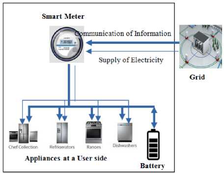
Fig.1. Demand side Energy Management with Storage Device

• A.    Problem Definition

The process of optimization is discussed only for one user as it is assumed that the same optimization process can be individually implemented at every user connected to the Grid. A user is assumed to be having a smart meter and some smart electrical appliances. There are two types of connection between the smart meter and the appliances. One is the power connection and the other one is a local connection (wired/wireless) for information communication between the smart meter and the devices. The smart meter contains a scheduler which generates an optimal schedule for the appliances and controls the operation of the appliances according to the generated schedule by sending control signals to them. The user has to feed the details about the appliances into the smart meter through some interface. The details can include the name of the appliance, its minimum and maximum power level, possible operation time, preferred operation time, kilowatt hour consumption rate, the minimum and maximum daily energy consumption amount and the preferred starting time of the appliances etc. As the smart meter is connected to the Smart Grid, it can get the required information from the Grid for a whole day like power cut timings and weather information etc., which can be used to calculate the optimal schedule. At the beginning of the day the smart meter uses all these information to calculate the operation schedule for the appliances using a GA/PSO based optimization algorithm. The pricing technique used here is TOUP according to which the user has to pay more prices during peak hours and less during off peak hours of the day. After generating the schedule the smart meter controls the operation of the electrical devices connected to the smart meter, according to the schedule.

• B.    Energy Consumption Schedule

As the scheduling is done for a whole day, a day is divided into some time slots. The total number of time slots in a day is considered as 24. One time slot consists of one hour. The total energy consumption for a particular hour of a user can be calculated from the amount of energy consumed by every appliance operating during that hour. Let e(h) denote the total energy consumed during hour h and e a (h) be the amount of energy consumed by the appliance a . The relationship between the two can be defined as:

e ( h ) = S ea (h ) (1) aeA

Where, A is the set of all appliances with the user. The amount of energy consumed by an appliance will be zero beyond its operation time described by the following constraint.

e_a ( h ) - 0, V h e H-H _a (2)

Where, H is the set of all time slots in a day and H_a is the set of all time slots in which the appliance a can operate. The total amount of daily energy consumption for an appliance a is represented as E_a which is calculated as:

E a = £ e a ( h )               (3)

h e H

As every appliance has a minimum power consumption level ( minp(a) ) and maximum power consumption level ( maxp(a) ), the hourly consumption of an appliance a is bounded by minp(a) and maxp(a) , which is described as:

minp ( a ) < e_a ( h ) < maxp ( a )             (4)

The energy consumption schedule for the whole day is represented through a vector e which can be described as:

e = [ e ( 1 ) , ...., e ( h ) , •••, e ( 24 ) ]                   ⁽⁵⁾

• C.    Energy Storage Schedule

The energy storage devices like batteries are used to help the user reduce energy consumption from Grid during peak hours. Let b be a vector that represents the charging or discharging schedule of the battery. It can be described as:

b = [ b ( 1 ) , ...., b ( h ) , ..., b ( 24 ) ]              (6)

When b(h) is -1 the user has to discharge(use) its battery energy. When it is 1 the battery is charged and when it is equal to 0 the battery is kept idle. Let L be the current charge level of the battery, C be the battery capacity and R be the charging/discharging rate of the battery. The charge level during a time slot h after charging or discharging has to satisfy the following constraint:

L min < L+ b ( h ) x R <  C, V h e H        (7)

It is further assumed that the energy level in the battery at the beginning of the day and at the end of the day remains at the minimum charge level denoted as L_min . The value of L_min is assumed to be 0 here. Thus the energy level at the beginning and at the end of the time horizon is kept at the same level. The following constraint ensures this condition,

2 b ( h ) x R-L min             (8)

h =1

Depending on the charging and discharging profile of the battery, during each time slot, the load to be bought from grid is defined as egrid(h) which has two components:

egrid ( h ) = e ( h ) + b ( h ) x R            (9)

• h. It is positive when battery is charged and negative when it is discharged. The total load demand from utility over the entire time of operation (one day) represented as LOAD which is calculated as:

LOAD = { egrid ( 1 ) +...+ egrid ( h ) + ...+ egrid ( 24 ) }   (10)

• D.    Objective of the System (Utility Maximization)

The objective of the proposed system is to optimize the user's satisfaction in consuming energy. The satisfaction of the user can be described as the utility the user gets from the daily usage of energy. So the objective can be described as the maximization of the value of the energy consumed by the user by minimizing the cost of energy and the level of dissatisfaction incurred by the user. The utility function is defined as follows:

.   . f                       24                                               1

Maximize V ^LOv4D^ — ^ C^ egrid (h ) ) — D^LOAD

I                r-1

Where, V(LOAD) denotes the value of the energy perceived by the user for the amount of energy equivalent to LOAD. The middle term represents the cost of total energy consumed during a day. D(LOAD) represents the level of dissatisfaction the user gets from the energy usage as a result of an unwanted operation schedule. That means the user gets some dissatisfaction when the scheduler does not schedule the operation of the devices according to its preferred time.

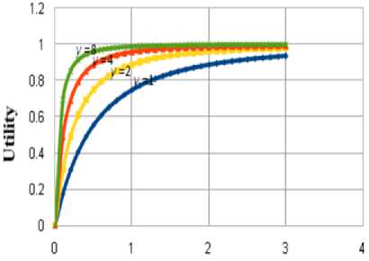
• •    Value of Energy is described as follows. A consumer's perceived value of a product or service is based on its theoretical ability to fulfil a need and provide satisfaction. In other words how much utility the user gets from the product determines the value of the product for the user. Similarly, the value of total energy consumed per day for a user can be described with the help of some utility function from microeconomics. A quadratic utility function has been used here whose value domain has been normalized between 0 and 1. The utility function for the total energy demand of the user for a day denoted as u(LOAD) is described as:

u ( LOAD ) = 1 — ( 1/ ( 1 + / x LOAD ) 2 )     (12)

Where, γ is a parameter representing the user's tolerance towards energy consumption curtailment. The utility function considered here satisfy all the properties of a valid utility function as the value of u(LOAD) is upper bounded by a positive value of 1, the first derivative u'(LOAD)>0 and the second derivative u" (LOAD)<0 .

e(h) is the amount of energy required for the appliances and b(h)×R is the charge level of the battery during hour

Resources

Fig.2. Utility Graph for Resources with different tolerance Level

The graph for the utility function is presented in Fig. 2. It can be seen from the graph that a utility function proceeds towards the upper bound slowly with a relative increase in the value of γ . The large values of γ indicate that the user is stricter with the energy reduction. Thus larger the value of γ lower the level of tolerance and lower the utility for the same amount of energy. The value of energy function can now be described as follows:

V ( LOAD ) = Unitp X LOAD x (1 - (1/(1 + у x LOAD )²))

• •    Unitp is the unit price that represents the value (in terms of money) for obtaining a unit of energy which is set by the energy supplier. It is equal to the average price of electricity in traditional pricing scheme where price remains fixed for each unit of electricity for the whole day. The unit price is taken from the traditional pricing scheme because it is assumed that the total cost of electricity for a day charged by the utility in the TOUP scheme is same as that of the traditional pricing scheme for the amount of same load. It is based on the fact that the value of the energy is not more than the average money the user gives for the consumption it makes in a whole day. LOAD is the amount of energy consumption in a day and the last term in the equation is the u(LOAD) used from (12).

• •    Cost of Energy is defined as follows. The cost that a user has to pay to the energy provider for the amount of energy consumed during a time slot h is denoted as c(egrid(h)) and the cost function is assumed to be an increasing function of the demand. That means the cost of energy consumption during time slot h is proportional to the amount of energy consumed during that slot. In most of the articles in the literature a quadratic function is used to define the cost function. But here a logarithmic cost function has been used. In case of a quadratic function the function value (i.e., cost) increases exceedingly when the demand varies extremely creating inconvenience for the

user at peak hours. However, the logarithmic function can give a near linear graph as it does not grow so fast with the demand. The energy cost function used here is defined as follows:

C ( egrid ( h ) ) = p x log ( 1/ ( 1 - x ) )        (14)

Where, p is the price coefficient or cost parameter whose value is more during peak hours (high pricing hours) and less during the off-peak hours that helps to control the consumption of the consumers during peak hours. The value of x is calculated as egrid(h)/k with the constraint 0, and k is a constant here.

• •    Dissatisfaction Level is expressed as follows. When the starting time of an appliance in the schedule generated by the smart meter matches with the user’s preferred time the user is fully satisfied that means the dissatisfaction level is zero. The level of dissatisfaction in fact depends on the difference between the scheduled stating time and the preferred starting time. A higher difference brings a greater level of dissatisfaction.

• IV.    GA Based Optimization

A detailed analysis of the GA based optimization technique has been presented in this section. The optimization tries to shift the loads from peak hours to off peak hours by generating an optimized schedule for the appliances based on the possible operation time of the appliances which reduces the energy price given by the user. The hourly load matrix is taken as the population on which the optimization has to be applied. Every individual in the population represents a possible candidate for the solution. The utility maximization function in (11) is considered to be the fitness function with the objectives to reduce the customers’ daily energy cost, reduce the peak power demand and increase the satisfaction level of the user. The simulation results given below provide an expansive idea about the optimization process.

• A.    Optimization with less consideration to the satisfaction level of the user

The following figures are generated from that part of the simulation where the scheduler generates the operation schedule for the appliances with little consideration to the dissatisfaction of the user that is caused due to delay in operation of the appliances.

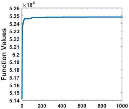
Fig. 3 shows that the algorithm converges after a number of iterations. Fig. 4 gives an idea about the energy demand pattern for the user before and after optimization. After optimization the maximum hourly consumption (energy demand from utility) during peak hours which was nearly about 8000watt is now reduced to 6000watt by shifting some of the load to non peak hours. It can also be observed that how the energy demand from the utility changes during 9AM to 12AM with the use of storage device. It is clearly visible that after optimization when the storage device is used the demand during these peak hours is further reduced. The battery is charged during non peak hours and provides energy during peak hours resulting less demand from utility during these hours. Fig. 5 shows the relative costs incurred from the energy consumption for a consecutive 24 days. It provides a comparison between the cost incurred before optimization and after optimization. It also depicts the effects and benefits of using the storage device. The graph representing the costs after optimization without the use of storage device remain low than that of the case with no optimization. The costs when optimization is performed along with the use of storage device are further reduced.

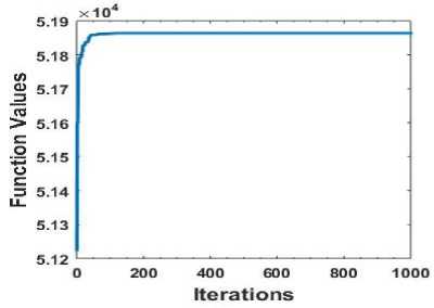
Fig.3.Convergence of the GA

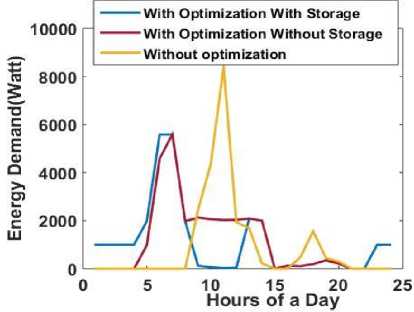
Fig.4. Daily energy demand with/without optimization

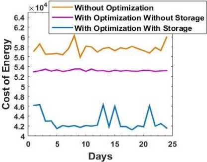
Fig.5. Energy costs for several days with/without optimization

• B.    Optimization with more consideration to the satisfaction level of the user

  In reality the user may get dissatisfaction when the appliances are not scheduled at its preferred time slots, so there is a need that the optimization should consider the satisfaction of the user. When the satisfaction level is increased in the optimization process the usage pattern is changed. However from Fig. 6 and 7 it can be seen that even after considering the dissatisfaction of the user in the optimization. From Fig. 6 it can be seen that the energy demand during peak hours is reduced when optimization is done and it is more reduced when storage is used. The costs of energy for several days are shown in Fig. 7. It shows that costs after optimization with storage device remain less than the other two cases where there is no optimization or optimization without using storage device. Fig. 8 and 9 represent energy demand for two different days. It is shown that when the consumption is scheduled according to user ’s preferred time the energy demand may be higher during peak hours than the case where less consideration is given to the user satisfaction level. For example during peak hours the energy demand may be around 3000watt when more consideration is given to the user satisfaction and near about 2000watt

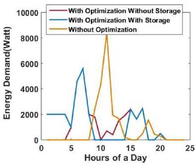
Fig.6. Daily energy consumption with/without optimization with reduced dissatisfaction level

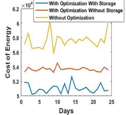
Fig.7. Energy costs for several days with/without optimization with reduced dissatisfaction level with reduced satisfaction. It leads to higher energy costs for the user as shown in Fig. 10. When the satisfaction level is high the cost of energy is also high as the usage during peak hours becomes high. So there is a trade-off between the cost of energy and the level of satisfaction. If the user wants to save cost then the satisfaction from the usage will be less and if the user wants to reduce the dissatisfaction then it has to give more cost for the same amount of energy it uses.

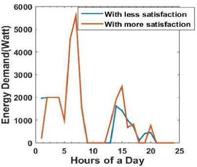
Fig.8. Energy demand with different satisfaction level

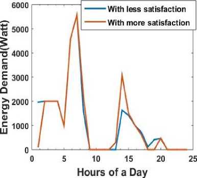
Fig.9. Energy demand with different satisfaction level

• V.    PSO Based Optimization

PSO is an evolutionary optimization technique which is inspired by the social behaviour of bird flocking, fish schooling and swarm theory. In this section the simulation results of PSO based optimization have been discussed. The following figures confirm the effectiveness of the algorithm. Fig. 11 shows the convergence of the PSO algorithm. Fig. 12 shows how the energy demand from utility becomes less during peak hours after optimization. From Fig. 13 it can be seen that the energy costs are less when compared to the scenario when there is no optimization. So PSO can be used as an alternative to GA.

In Fig. 14 and 15 comparisons are made between the cost graphs for a consecutive 25 days generated by the optimization algorithms GA and PSO. Fig. 14 shows the result of the simulation where the random state is fixed and Fig. 15 is the result of the simulation where the random state is not fixed. It is to be noted that in fixed random state when the algorithm is executed repeatedly the environment generates same random numbers and if the state is not fixed the set of random numbers generated during each execution is different. In both the cases the costs calculated by PSO are less than the costs given by GA for all the days. It can be noted from Fig. 3 and 11 that the values of the objective function calculated by PSO are greater than the values calculated by GA. A statistical comparison between PSO and GA based on the results of the simulation can be found in Table 1. The resultant fitness values of 60 independent runs of each algorithm are taken for comparison. The first 20 executions are done with a population of size 10 for 1000 iterations (generations). The second 20 executions are done with a population of size 10 for 2000 iterations. The third 20 executions are done with a population of size 20 for 1000 iterations. It can be seen that the minimum, maximum and mean of the fitness values calculated by PSO are larger than the minimum, maximum and mean calculated by GA. From these generalizations it can be considered that performance of PSO is better than GA for the proposed technique.

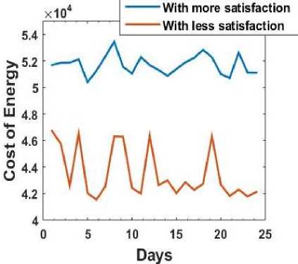
Fig.10. Energy costs for several days with different satisfaction level

Iterations

Fig.11. Convergence of the PSO

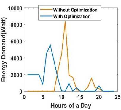
Fig.12. Daily energy demand using optimization by PSO

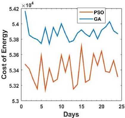
Fig.14. Energy costs for several days with random state fixed

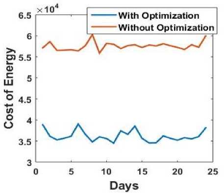
Fig.13. Energy costs for several days using optimization by PSO

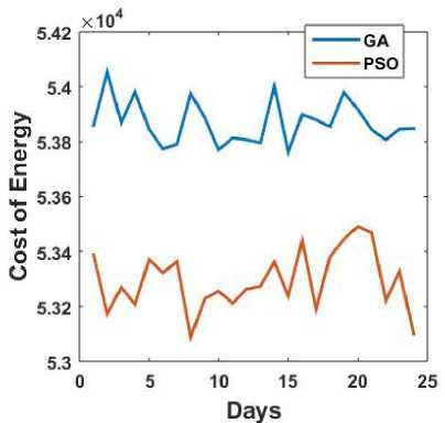
Fig.15. Energy costs for several days with random state not fixed

Table 1. Performance of PSO versus GA

Statistical Measures of Fitness Values	Maximum	Minimum	Mean
GA with population size 10 and 1000 iterations	5.19E+004	5.16E+004	5.18E+004
PSO with population size 10 and 1000 iterations	5.26E+004	5.19E+004	5.24E+004
GA with population size 10 and 2000 iterations	5.20E+004	5.17E+004	5.18E+004
PSO with population size 10 and 2000 iterations	5.26E+004	5.21E+00	5.24E+004
GA with population size 20 and 1000 iterations	5.20E+004	5.18E+004	5.19E+004
PSO with population size 20 and 1000 iterations	5.26E+004	5.19E+004	5.22E+004

• VI.    Rising Peaks During non Peak Hours

From the simulations it is clear that most of the consumption is shifted to non peak hours when optimization is implemented. It is clear from the Fig. 4 and 6 that the consumption becomes very high during off peak hours due to optimization. As the price of energy is less during non peak hours the optimization process tries to shift maximum possible load to non peak hours. When every user in the system tries to shift most of its consumption to non peak hours without any limit on hourly the consumption amount it may increase the total load in the system during these non peak hours. However shifting of loads may result in a scenario where there is a possibility of rising peaks in the off peak hours. It may again create imbalance between the demand and supply of energy. The market price of energy during these hours may also be increased to fulfil such high demand which finally has to be incurred by the consumers. Due to high demand the Grid may also become unstable. So for the flawless working of whole Grid system it is better to put some limit on the amount of hourly energy demand made by the users. This constraint has been included in the simulation and the following figures confirm that when the user's demand for energy from the utility is less or equal to the limit set for the hourly demand amount, the peak demand is reduced along with the shifting of maximum possible consumption to non peak hours keeping the demand graph somewhat flattened which leads to reduced cost of energy and well maintained balance between demand and supply of energy due to optimization. As a result the Grid remains stable and become more reliable. In Fig. 16 it is shown that when the peak reduces the demand graph becomes smooth. The demand of near about 6000watt reduces to a demand of around 3500watt. Fig. 17 confirms that the cost of energy remains high when the demand becomes high. The reason behind this is the value of the cost parameter p used in the cost function (14) is more during high demand hours yielding high cost of energy. So the overall cost happens to be less when the demand is less.

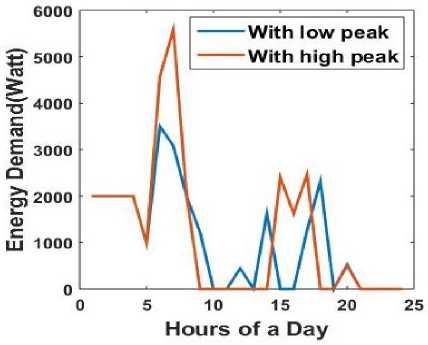
Fig.16. Daily Energy Demand With/Without High peak

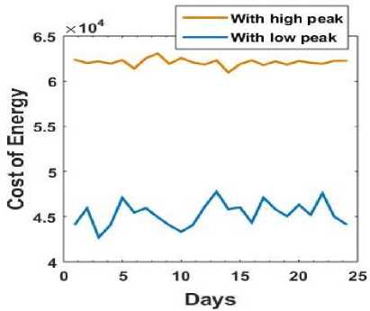
Fig.17. Energy Costs for Several Days With/Without High peak

• VII.    Conclusion

Shaping the Energy Demand curve is the main objective of this work that is executed through load shifting along with the use of storage device in the presence of a TOUP tariff. The proposed method helps in smoothing the demand profile and reducing the peak demand by motivating the users to shift some of the load from high-peak to low-peak hours which will diminish largely the plant and capital cost prerequisites and the cost of the generated energy. In addition to this it will enhance the system reliability. The proposed approach also tries to accomplish a trade-off between minimizing the electricity payment and reducing the level of user dissatisfaction caused due to delay in time for the appliances’ operations. Simulation results confirm the effectiveness of the proposed approach. The evolutionary optimization techniques like GA and PSO have been used to determine the optimum demand pattern for the user. A comparison between the results obtained from the optimization using these algorithms individually has been introduced. The comparison helps to assess the reasonableness of the proposed optimization system. Both the algorithms work more or less in a similar fashion. However PSO appears to be a better option than GA for the given optimization process which is confirmed from the simulations. The optimization technique is able to implement an efficient DSM system that meets the user requirements and schedules the operations of the electrical appliances for the whole day which improves the electricity consumption behaviour of the users. The benefit of using storage devices is also highlighted in this work. By using the storage unit the users can get more economical advantages. It is to be noted that further improvements could be acquired if the proposed energy management strategy would be adaptive to the unexpected behaviour of the consumers in energy demand and if it could include features to handle renewable energy resources. Development of such DSM technique is planned as a future work of the authors.

Nilima R. Das did her M.Tech. in Computer Science and Engineering from Utkal University, Odisha in 2008. She is currently pursuing her Ph.D. from Siksha ‘O’ Anusandhan, Deemed to be University, Bhubaneswar, Odisha.

She is working as an Assistant Professor in the Department of Computer

Applications, Institute of Technical Education and Research,

Odisha. She has published 3 International Journal papers.

Satyananda C. Rai did his M. Tech. and Ph.D. in computer science and Engineering from Utkal University in 2001 and 2012 respectively.

He is currently working as an Associate Professor and head of the Department of Information Technology at the Silicon Institute of Technology, Bhubaneswar. He has published 23 research articles in national and international conference proceedings as well as in journals. He has written a monograph titled QoS Provisioning in Mobile Ad Hoc Networks: Principles, Practices and Models, published by LAMBERT Academic Publishing, Germany in 2013 and co-authored a book titled Computer Network

Dr. Rai is a member of IEEE, a life member of Indian Society for Technical Education (ISTE), Indian Association of Medical Informatics (IAMI), and Orissa Information Technology Society (OITS).

Ajit K. Nayak has done his graduation in Electrical Engineering from the Institution of Engineers, India in the year 1994, M. Tech degree in computer science from Utkal University in 2001 and Ph. D Computer Science from Utkal University in 2010.

He is the professor and HoD of the Department of Computer Science and