Interative-phase method for diffractively levelling the Gauss beam intensity

Author: Golub М.А., Doskolovich L.L., Kotlyar V.V., Nikolsky I.V., Soifer V.A.
Journal: Компьютерная оптика @computer-optics
Section: Численные методы компьютерной оптики
Article in issue: 13, 1993.
Free access
The phase diffractive optical element that transforms the Gaussian collimated beam into the uniformly illuminated rectangle has been calculated. In computing the phase function we have employed an adaptive iterative algorithm which is generalization of the Gerchberg-Saxton method. The smooth phase function derived using geometrical optical methods has been used as an initial approximation.
Short address: https://sciup.org/14059574
IDR: 14059574
Text of the scientific article Interative-phase method for diffractively levelling the Gauss beam intensity
The demand for optical elements capable of levelling the Gaussian intensity distribution exists in such problems of optical data processing as laserbased superficial strengthening and laser projection printing. The diffraction redestribution of the light beam intensity can be performed by means of so called focusators of laser radiation [1,2]. Methods of geometrical optics make it possible to derive [2,3] analytical relationships for a focusator phase which is the smooth function of two variables. However, such an approach ignores diffraction effects that can result in low accurace in formation of the required focusator-produced intensity distribution. On the other hand, in computing a phase of kinoforms, an iterative algorithm [4-6] is employed, which takes into account diffraction effects taking place under the light propagation. Making use of the adaptive correction procedure [7,8] allows this algorithm to be successfully applied to compute the phase of focusators.
This paper deals with numerical comparison of performances of focusators from the Gaussian beam into the uniform intensity square computed by geometrical-optical with those computed by iterative methods.
-
2. Focusing from the Gaussian beam into a rectangle
As it has been shown [9], for the focusator that form the rectangular intensity-uniform distribution as
K*.yV
1. Msd,,
0, |x|>d1(
|y|^
|У|>^2
from the plane beam with the Gaussian profile of the intensity distribution
Ци^=10ехр-У—- , we can (given a lens located immediately adjacent to the focusator) find its phase function in the form of the sum ф^Л^фДи^ф^у) , with its terms satisfying the set of two simultaneous equations dx № du /(x) x-.^fk'^l , du where /is the focal length of the lens in whose focal plane the light rectangle is formed, к is the wavenumber of light, (u,v) and (x,y) are the coordinates in the planes of the focusator and of the Fourier spectrum, respectively, 2^, and 2d2 are the measures of the rectangle and a is the parameter of the Gaussian beam.
The first equation in the system (1) sets the equality of the density of light energy of a ID focusator to the density in the corresponding areas of the straight-light segment. The second equation in the system (1) describes the stationary points in the paraxial approximation.
The discrete variant of the solution of the system (1) can be written as follows
Фтп=1п(10) MAenN-'ert^nN-'V
-i ll m
+п гехр(-36л2Л/-2)^Му6тА/-1х xerf^mNf^ 2ехр(-36тгЛГ2)( , where erf(x)=2tt 2Jexp(-t2)dt , о m=0,±l,±2,...,±jV/2, n=0,±l,±2.....±NA. M^Nx^^AQY\ M^N^^AQY\ M. and Nf are the number of the minimum diffraction spots that fall into the rectangle with the measures NxxNv In this case, the square aperture of the focusator measured NxN equals to the measure of the square, 6a, and the Gaussian collimated beam that illuminates the focusator produces the light distribution as lOmn-ex^ 36N"4n2*m2^ (3)
In section 4 we employ the phase (2) to numerically simulate the operation of a geometrical-optical focusator.
-
3. Adaptive-iterative computation offocusators
Following [7,8], let us briefly describe how the iterative algorithms can apply to computing the focusators as kinoforms. Let us proceed from the preset complex amplitude .4(1/) of the illuminating beam and the required intensity distribution /(.x) in a focal plane of the lens. The complex amplitude Дх) in a focal plane is related to the complex amplitude
/(и)=а(и)ехр[/ф(и)]
immediately behind the focusator through the Fourier transform
ь
Rx)=J f(u) exp(/kxu/f)dx,
-b where lb is the size of the focusators aperture. The focusator's equation takes the form
№)|2=/(x) <4)
To find iterative solution of Eq.(4) with respect to the phase ф<и\ one should perform some preliminary estimate of the phase ф0(н) followed by the computation of the complex light amplitude in a focal plane. In this case the complex amplitude Fn(x) calculated in the и-th step of iterations is replaced by the function F^x) according to the rule
I VWF„(x)|Ffl(x)r\ |x|.d
I “2F„(x) , |x|>d where /п(л)=(1 + a)I(x)-a |Д(х) |2, /(.x) is the required intensity distribution within the interval |-d,d| of a focal plane, a is the parameter that controls the rate of convergence of the calculated intensity to the required one. For «=0, the replacement (5) changes to the standard replacement in the Gerehberg-Saxton algorithm [5].
The amplitude of light in the plane of focusator Д(и) is calculated with the help of the inverse Fourier transform and is replaced by the function Л°(-х) according to the rule f°nW=
А1иУпЦЛ№КА , |v|sb (6) 0 , M>b .
In contrast to the algorithms of the conditional gradient [10], the a parameter is here introduced directly into the intensity function.
The rate of convergence of the intensity |Fn(x)|2 to the required one /(.x) is checked by the root-mean-square deviation
[/[/(х)-|^(х)№
1/2
6 =
-d
d f /2(x)dx
-d
Besides, a new parameter e characterizing energy efficiency of focusing is introduced:
the
/№)|2dx e^ —
[ \адм
In the next section we apply the phase derived from Eqs. (4)-(6) to numerically simulating the operation of diffractive focusators.
-
4. Numerical results
We examine the focusator into a square that comprises 32x32 pixels and measures 10 minimum diffraction spots. For a focusator that focuses from the Gaussian collimated beam into a square, the phase deduced from Eq.(2) on the net of pixels 256x256 and
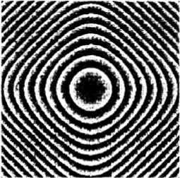
Fig. 1 Geometrical -optical phase og the focusator into a square.
taken to the modulus 2k represents the set of rings
(lines of equal phase) changing to the lines of the square perimeter (Fig.l). Figure 2 illustrates the light intensity distribution in the lens focal plane calculated as the Fourier transform of the amplitude
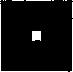
i------^--- Fig.2 The intensity distribution ^mn=vbmn® ™ , obtained iron the geometrical-where is taken '““',n ’'™ tol from Eq. (3) and фтп from Eq. (2). The root-mean-square deviation of the obtained distribution from the uniform one amounted to 5% and the efficiency was 91.6%.
To calculate the focusator that focuses the Gaussian beam into the uniform intensity square, as an initial phase estimate we have chosen the geometrical-optical phase function described above (Fig.l). The subsequent iterative calculation has been conducted using three techniques. Ute first approach to the calculation of the phase based on the standard variant of the Gerchberg-Saxton algorithm with the replacement (5), for «=0, yields, at first, the increase of the error <5 in the first iteration steps and then it gives the slow decrease of the error (Fig.3a, curve 1). In this case during 10 iterations the error does not diminish below 13% though the efficiency e grows up to 98.9% (Fig.3b, curve 1).
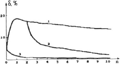
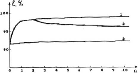
Fig.3 The root-mcan-square deviation (a) at the energy efficiency (b) agains the number of iterations for different variants of an iterative algorithm: Gcrchbcrg-Saxton (1). combined (2), and adaptive (3).
The second approach is combined: the first three iterations are conducted with the replacement (5) for a-0, the remaining seven iterations for a=l (Fig.3a, curve 2). This method after 10 iterations results in formation of the square characterized by the uniform intensity, with the error of 2.4% and the efficiency of 96.4% (Fig.3b. curve 2). This way is seen to be more effective as compared with the first approach, since it yields the decrease of the error from 13% to 2% (by 6-fold) without essential decrease in the efficiency.
The third method is purely adaptive, this means that the replacement (5), with a-1, is performed in each step of iteration (Fig 3a, curve 3). As one can see in this case, the error decreases monotonously and during 10 iterations it becomes equal to 0.1%, but the efficiency falls to 92.2% (Fig.3b, cur-
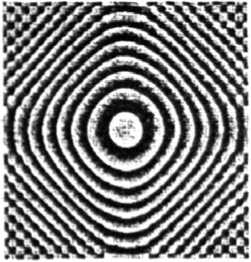
Fig. 4 The phase of the focusator into a square obtained after 10 iterations from the initial geo-metro-optical phase.
ve 3). Figure 4 illustrates the phase of the focusator to the modulus 2я that has been calculated during 10 iterations on the basis of the third approach from the geometrical-optical phase (2). First, one can see that the use of the iterative algorithm does not result in the essential change of the initial phase The pronounced changes of the phase
(Fig.l) take place only on the edges of the focusator (Fig.4). Second, we can draw the conclusion that the adaptive iterative algorithm based on the replacement (5) for a=l makes it possible to improve the geometrical-optical phase in such a manner that the error in the formation
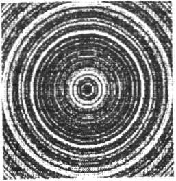
Fig.5 The radius-random phase chosen as the initial estimate for iterations.
of a light square reduces more than by an order, with the efficiency almost unchanged.
For the aim of comparison, there was conducted another numerical simulation where we made use a radius-random phase function (Fig.5) as the initial approximation. The phase shown in Fig.6 was calculated during 10 iterations. The intensity distribution formed by the focusator characterized
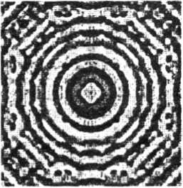
Fig.6 The phase of the focusator into a square obtained after 10 iterations from the initial random phase.
by such a phase is presented in Fig.7. The error and the efficiency were equal <5=6.4% and e^80.8%, respectively. Further iterations did not produce the essential change in these values. Data given above show that the iterative algorithm that begins with the random phase estimate, leads to the non-regular structure of the focusator's zones and results in the
Fig.7 The intensity distribution in a lens focus obtained from the focusator with a phase shown in Fig.6.
accuracy and efficiency which are somewhat less than those for a geometrical-optical focusator.
The table summarizes all the focusators discussed in this paper. One can see the advantages tn terms of the uniformity, the efficiency, and the regular phase structure that we achieve when using physically warranted initial approximation in the form of the geometrical-optical phase (compare rows 1-4 with row 5). The comparison between rows 1 and 2 in the table shows that the Gerchberg--Saxton method yields the increase of 7% in the energy efficiency of the geometrical-optical approximation (row 1) but produces considerable non--
Table
