Interval explosion search algorithm and its application to hypersonic aircraft modelling and motion optimization problems

Development of hypersonic aerial vehicle (HAV) control techniques is very urgent field of applied cybernetics [1]. One of possible opportunities consists in spaceplane creation. Spaceplane is a special type of spacecraft which can soar and hurtle as an ordinary plane. In consequence of principally different interaction between HAV and atmosphere all proposed methods should be analyzed accurately to find out advantages and disadvantages. To raise accuracy it is important to develop new numerical methods using metaheuristc and interval optimization algorithms [1-3], which can give an appropriate solution for the HAV optimal open-loop control problem.

Existing numerical methods of optimal control include various methods which use Pontryagin’s maximum principle and Bellman’s equation, direct methods (e.g. gradient methods, first-ordered methods), second-ordered methods which are based on a Taylor appoximation of Krotov - Bellman function, different improvement methods and etc. [4,5]. There is a need in development of new approaches in order to improve the efficiency and accuracy. Such an approach consists in the use of interval analysis coupled with metaheuristic strategies [2,3].

Interval analysis [6-10] is used as the main component of interval explosion search (IES). Existing interval optimization methods can be divided into a few groups:

e methods of unconstrained optimization (Moore - Skelboe algorithm, Ichida - Fujii algorithm, Dussel algorithm, interval simulated annealing, graph subdivision method and etc. [11-13]), e methods of constrained optimization (Hansen method, Moore method and etc. [7,9]).

IES belongs to the group of so called metaheuristic algorithms. Metaheuristic algorithms give admissible solutions in the most practically significant cases. Such algorithms do not guarantee obtaining the best solution, but the main advantage is that they have lower computational complexity. Thus they can be applied to complicated problems without additional constraints on problem statement (differentiability, convexity and etc.). Also these methods do not use necessary and sufficient optimality conditions [1]. Metaheuristic algorithms combine one or several heuristic procedures which base on the higher level strategy.

In the following work it will be shown how general open-loop control problem can be transformed into the form of interval constrained global optimization problem which will be solved numerically with the IES. Method efficiency is demonstrated on the solution of HAV optimal control problem.

1.    Interval Analysis. Definitions and Notations

The main idea of interval analysis [6-10] is that real numbers are surrounded with intervals and real vectors - with interval vectors, or boxes. Hereafter, lowercase letters in square brackets ([ a ] = [ al ; au ]) will be used to denote intervals and bold lowercase letters in square brackets ([a] = [ a 1] x ... x [ an ]) - for boxes.

Each interval has the following characteristics:

• •    lower 1 round: [a] = sup {C G R U {to. to} |VZ G [a] : C < Z}

• •    upper bound: [a] = inf {C G R U {—to, to} |VZ G [a] : Z < C}•

  [ a ]+[a ]

  2     •

  
  

• •    width of nonempty interval: ш ([a]) = [a] — [a];

2.    Interval ^-Minimization Problem

midpoint of nonempty and finite interval: mid ([ a ]) =

The same parameters are defined for boxes. Lower and upper bounds and midpoint become vectors, width is now calculated as maximum of component’s widths.

Interval hull of a set X C R ⁿ Is the smallest box (box with minimum width) [X]. that contains X. If the set is surrounded by square brackets it means that we consider the interval hull.

Let о Ire a binary ojrelation. then [ x ] о [ y ] = [ {C 1 о C ₂ |C 1 G [ x ] . C ₂ G [ y ] } ]: 1 et f Ire an unary operator, then f ([ x ]) = [ {f ( C ) |C G [ x ] } ].

The set of intervals is designated by IR, set of boxes - by IR ⁿ . Consider a function f from R ⁿ tо R. The interval function [ f ] from IR ⁿ tо IR is an inclusion function for f if V [ x ] G IR nf ([ x ]) C [ f ] ([ x ]). Inclusion function allows to get a priori estimate of function’s range even if it is nonconvex or disconnected. If all variables are substituted with intervals and all operations are done by the rules of interval arithmetic such a value is called an estimation of a direct function image.

Consider a given box [s] and a, cost function f : Rn ^ R. luterval e-minimizatioii problem consists in determination of such a box [p]* C [s] that ш ([p]*) < e. @ [x] C [s].ш ([x]) > e[f] ([x]) < fOpf)                 (1)

where the value e affects the лvldtli of the [p] * box.

3.    Strategy of Interval Explosion Search (IES)

During the initialization bombs are randomly placed on the search area. Each bomb is associated with the box which describes its location. Moreover, all bombs are sorted (by ascending) by the lower bound of its direct function image estimation. IES has two iterative phases (Fig. 1): global and refining search, which differ from each other by the explosion procedure realization. Each iterative phase consists of:

• 1)    bomb power calculation (power vector affects splinter scatter radius),

• 2)    explosion procedure (during this procedure each bomb produces two splinters (new interval vectors) which scatter into different directions),

• 3)    bomb list renewal.

4.    IES Algorithm

Algoritm terminates when the maximum number of iterations is exceeded. From the bomb list we choose the one with the minimum lower bound of its direct function image estimation.

Fig. 1. IES strategy

Step 1. Set iteration number tg = 0, maximum number of global and refining search tmax ai 1(i tmax- maximum nuiuber of bombs Bmax. power vector rmax € Rn. searcli area [s] tgmax +tcmax and e = 2 n     • ш ([s]).

Step 2. Randomly distribute bombs (interval vectors) on the search area: {[b] = [C 1; Z 1 ] x • •• x [Cn; Zn]}BTxi where Cj and Zj are random numbers which are uniformly distributed over interval [sj] (if Cj > Zj^ then the corresponding interval is substituted with the interval [Zj; Cj])• Sort bombs by ascending of the lower bound of the direct function image estimation.

Step 3. Bomb power calculation. For each bomb [b]i from the list calculate its power i-1

B max ^- 1

vector: pi =

• ^r max * i 1 , •••, ^B max •

Step 4. Explosion (global search). During this step each bomb produces two splinters by the bisection procedure. Bisection is a division along the widest component [8]. Thus we obtain two new bombs from the given one: [b]i =

[ b 1] i

^{6 (} -p l; p l)

//[ b 1] Л

^[ bk ^] i

[ bn ] i

+

^{all(1 [Ь]} B max+ i

^[ bk ^] i

[ bn ] i

+

6 ( -pk ;0)

^{6 (} -pn ; pin )

F l [s]. wlieie 6 ( a ; b )

/ ^{6 (} -p l p l) XX

6 (0; pk )

^{6 (} -pn ; pin )

П [s]

is a random variable

uniformly distributed on interval [ a ; b ], k = Arg max ш ([ bj ] ). j =1 ,...,n           ⁱ

Step 5. Bomb list renewal. On the previous step number of bombs has been doubled. Thus unnecessary ones should be removed: sort bombs in ascending order by the lower bound of the direct function image estimation. Remove last Bmax bombs.

Step 6. Increase tg bу 1. If tg < tg max then return to step 3, otherwise go to step 7.

Step 7. Set iteration number tc = 0.

Step 8. Bomb power calculation. For each bomb [b] i from the list calculate its power X ep     в max _1 • rmax- i    ¹, ...,B max

Step 9. Explosion (reining search). During this step each bomb produces two splinters by the bisection procedure. Bisection is a division along the widest component [8]. Thus

/7[ ^b 1] Л

/ 0 w

we obtain two new bombs from the given one: [b] i =

[ b 1] i

B max+ i

^[ bk ^] i

\ [ bn ] J

+

6 ( -pk ;0)

^[ bk ^] i

\ [ bn ] ,/

+

6 (0; pk )

П [s]. k = Arg max ш ([ bj ].). j =1 ,...,n           ⁱ

П [s] and

Step 10. Bomb list renewal. Sort bombs in ascending order by the lower bound of the direct function image estimation. Remove last Bmax bombs.

Step 11. Increase tc bу 1. If tc < tC max then return to step 8, otherwise go to step 12.

Step 12. Choose the box which is associated with the bomb with the smallest lower bound of the direct function image estimation as a problem solution [p] * . Find [ f ] ([p] * ) as a cost function interval.

5. Optimal Open-Loop Control of Continuous Deterministic Systems

Behaviour of control object is described by differential equation [16]:

^x(t ) = f ⁽ t,x ⁽ t ) ,u ⁽ t )) ,

where t E T = [ t о; t 1] is contlnuous time. T is the system operational time, x E R ⁿ is the system state vector, u E [u] C R q is a control vector, [u] is a set of admissible control values (box), f ( t, x,u ) = ( f 1 ( t,x,u ) ,...,fn ( t,x, u ))^T is a continuous vector-function.

Initial state is given x (t0) = xо.(3)

Terminal state x ( t 1) should satisfy the following interval terminal conditions:

Г i (x (t1)) E [ Gi ] ,i = 1 ,...,l,(4)

where 0 < l < n, [ Gi ] are given intervals, funotions Г i ( x ) are continuously differentiable, system of vectors ^{д r} i ^{( x} ) ,..., ^{d r} i ^{( x} ) , i = 1 ,..., l is linearly 1 ndependent Vx E R ⁿ.

∂x1

The only information which is used to form control is continuous time t . Hence we consider open-loop control.

Set of admissible processes D ( 1 ₀ , x ₀) is defined as a set of pairs d = ( x ( ■ ) , u ( ■ )) which Include trajectory x ( ■ ) and adriiissible control u ( ■ ). where Vt E T : u ( t ) E [u] and state equation (2), initial condition (3) and terminal condition (4) are satisfied.

On the set of admissible processes we consider cost functional

I

( d ) = f ¹

t 0

f ( t, x ( t ) , u ( t )) dt + F ( x ( 1 1)) ,

where f ⁰ ( t,x, u ) and F ( x ) are given continuous functions.

In order to transofrm the given problem into a problem without terminal constraints (4) we can use penalty function:

l

I ( d )= I ( d ) + ^ Ri ¹* ■ H«,                         (6)

i =1

where H^ = hу ([Г i ( x ( 1 1)); Г i ( x ( 1 1))] , [ Gi ]). h^ ([ a ] , [ b ]) = inf {r| [ a ] C [ b ] + [ -r ; r ] } Is a Hausdorff metric, R^ are penalty parameters.

If there are interval phase constraints {pj ( x ( t ) , u ( t ) , й( t ) , u ( t )) E [ Pj ] , Vt E T}j = 1, where pj ( ■ ) Is the constraint function. [ Pj ] are given intervals. N_p Is the number of constraints, then we have another form of modified cost functional (5):

l                   N p

I ( d ) = I ( d ) + £ R" ■ Hi¹¹ + £ R* ■ H®,               (7)

i =1                 j =1

where t1

^Hj ⁽²⁾= 1^h ^ ^([ pj ^{( x (} t ) ^{,u (} t ) ^,:x ⁽ t ) ^{,ui (} t )); pj ^{( x (} t ) ^{,u (} t ) ^,:x( t ) ^{,ui (} t ^))] , ^[ Pj ^{]) dt}, t 0

Rj ²^ are penalty parameters.

The problem is to find such a pair d* = ( x* ( ■ ) , u* ( ■ )) = arg min I ( d ).

dED ( 1 0 ,x 0)

6. Application of Interval Optimization Technique

We will consider interval control as a piecewise-constant or piecewise-linear interval function [ u ] ( t ) and interval trajectory as a piecewise-continuous interval function which satisfies (2) - (4).

The piecewise-constant control (Fig. 2 (a)) can be uniquely associated with an interval

vector [ u 1 ( т ₀)] x ... x [ uq ( т о)] x... x [ u 1 ( TN - 1)] x ... x [ uq ( TN - 1)], wlicre Ti =

|

^^{z^“ ^{[ u ( T} о ^)]

}      |

{Z

^{[ u ( T} N - 1 ^)]

}

t i ^-t о . ; t 0 ⁺ N

and N is number of discretization steps. Corresponding interval control can be found as follows: [ u ] ( t ) E [ u ( т )], т < t < т_{i +1}. i = 0 ,..., N — 1.

The piecewise-linear control (Fig. 2 (b)) can be uniquely associated with an interval

vector [ u i ( т 0)] x ... x [ uq ( т 0)] x... x

[ u ₁ ( TN )] x ... x [ uq ( t _n )]. Corresponding interval

|

}

|

}

E

^{[ u ( T} 0 ^)]

"V

^{[ u ( T} N ^)]

• ^{[ u (} T ^)] +

-t

—i- • [ u ( Ti +1)], Ti < t < Ti +1.

control can be found as follows: [ u ] ( t ) i = 0 ,...,N — 1.

-τ i

(a)

(b)

Fig. 2. Piecwise-continuous interval control

It is suggested to find the interval vector, which satisfies condition (1), by the IES algorithm (optimization will be done on the search area [s] = [u] x ... x [u] for the

|---------z---------} q·N piecewise-constant interval control and [s] = [u] x ... x [u] for the piecewise-linear interval

|---------z---------} q-( N +1)

control).

The value of the cost function criterion (14) is calculated by the numerical methods using Euler, Euler - Cauchy or Runge - Kutta formulas [3] (all calculations on the right hand side of equations are done by the rules of interval arithmetic [6-10].

7.    HAV Optimal Open-Loop Control Problem

Consider the following system of differential equations [17] which describes HAV landing process:

/

^{y (} t ) =

Ω ² ·t

⁺ V

r (t) _ V • sin y, ф (t)   V• cosy*sin Ф

Lc^ + ( V — V ) + r 2 • О • cos ф • cos ф + m·V       r V

■ cos ф • (cos y • cos ф + sin y • sin ф • sin ф ) ,

V ( t ) = -D m

L·sin σ ф v)    m-V• cosY

^^^^^^^^^r

0 (t)   V• cos Y*cos Ф r·cos ϕ , g • sin y + 02 • t • cos ф • (sin y • cos ф — cos y • sin ф • sin ф),

^^^^^^^^^r

V • cos y • cos ф • tan ф + 2 • О • (tan y • cos ф • sin ф — sin ф ) — — ^Q 2 • t • sin ф • cos ф • cos ф,

V · cos γ

where r is the distance from the Earth center. 0 is the longitude, ф is the latitude. V is the Earth-relative velocity, y is the flight path slope, ф is the velocity azimuth angle, a is the roll angle, g _ GM is the acGM is the Earth gravitational constant. О is the Earth rotational velocity, m is the HAV mass, L _ 2 • p0 • ( ^e(r-r0)‘ V²• C_L • Sref is the aerodynamic lift force, D _ 2 • p0 • ₍^e(r-r0)V²• C_D • Sref is the aerodynamic drag force, p 0 is the sea-lev el air density, в is the numerical coefficient, p 0 is the numerical constant, CL, C_D are the aerodynamic force coefficients, Sref is the HAV surface area.

The aerodynamic force coefficients are defined by a polinomial function of Mach number M _ V (V_s is sonic velocity) and attack angle a basing on X-33 project information:

C_L _ — 0 , 0005225 • a ² + 0 , 03506 • a — 0 , 04857 • M + 0 , 1577 , C d _ 0 , 0001432 • a ² + 0 , 00558 • a — 0 , 01048 • M + 0 , 2204 .

The numerical parameters which are used in the model: m _ 35828 кg, Sref _ 149 , 3881 in 2. p о _ 1 , 2256 kg in³, r о _ 1 , 2256 ni. в _ 0 , 00013785 iii ^- к GM _ 3 , 986 • 10¹⁴ in³ /s ². О _ 0 , 000072722 rad s. Re _ 6378100 ni. V_e _ 11180 m s.

The state vector consists of 6 components: x ⁽ t ) ^{_ ( r (} t ) ^{,0 (} t ) ^{,ф (} t ) ^{,v (} t ) y ⁽ t ) ^{,ф (} t )) T- The HAV control is realized by attack and roll angles: u ⁽ t ) ^{_ ( a (} t ) ^{,a (} t )) T-

The initial state of the system: r ( 1 0) _ 6429100, 0 ( 1 0) _ — 85, ф ( 1 0) _ 30, V ( 1 0) _ 2600. y ( t о)_ — 1 , 3. ф ( t о) _ 0.

The HAV control vector:

u (t) _ (a (t), a (t)) G [ —10; 50] x [—80; 80] , Vt G T _ [0; 530] .(10)

The terminal conditions:

r ( 1 1) G [6378578; 6378822] , V ( 1 1) G [91 , 44; 91 , 44] ,

0 (11) G [—80, 7126; — 80, 7098],      y (11) G [—6; — 6],(11)

ф ( 1 ₁) G [29 , 998903; 30 , 001097] ,    ф ( 1 ₁) G [ — 60; — 60] .

The HAV trajectory phase constraints:

q ( t ) G [0; 14364 , 1] , h ( t ) _ r ( t ) — Re G [0; 121920] , V ( t ) G [0 , 3; 5200] ,

Q (t) G [0; 242000] ,               0 (t) G [—90; 90] ,            y (t) G [—89; 89] ,(12)

ngg (t)_ nnzf G [—2, 5; 2, 5] ,          ф (t) G [—89; 89] ,          ф (t) G [—180; 180] , where q = | • p0 • e e(r ro) • V2 is the dynanhe pressure. Q = 4,477228 • 10 9у/p0 • e e'(r ro) • V3,15 is tire lieat rate. n = Lcosa+Dsina| is normal acceleration.

zm

The constraints on control vector rate:

<» ( t ) e [ - 5; 5] ^ ^{a (} ’ p 1 - a^{T i )} e I - 5; 5] , о ( t ) e I - 5; 5] ^              e [ - 5; 5] .

The cost functional for the given problem:

I(d) = ЁR1’ • H^ + ЁR*7 • H?’,< i=1

where RJ1) = 1000. RJ1) = R= R((1) = RJ1) = 1000000. RJ1) = 10000 arid R(2) = R(2) = 1        2    3    5    6          414

• ( 2)       (2)             (2)       (2)       (2)       (2)       (2)                  (2)(2)

• 7  —  8  —     2  —  3  —  5  —  6  —  9  —         10 —11 —

It is required to find time histories of attack and roll angles, which minimize cost functional (14).

IES was implemented in a software complex, Visual Studio IDE and CT programming language. Parameters of the IES: tf _nax = tC _nax = 2500, B _max = 100, r _max = 0 , 05 for each dimension.

Charts on Fig. 3 show the results from [17] which were obtained by B-splines and Galerkin projection technique.

Fig. 3. State vector components

Charts on Fig. 4, show the results for the piecewise-constant interval control.

Charts on Fig. 5 show the results for the piecewise-linear interval control.

Information about constraints satisfaction are represented in Tables 1, 2.

Thus, by comparison of the results we can conclude that IES algorithm can be efficiently applied to HAV optimal open-loop control problem. Obviously it is better to

Fig. 4. State vector components

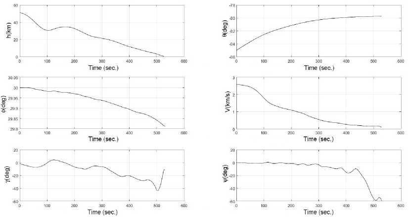
Fig. 5. State vector components use piecewise-linear control to satisfy constraints more accurately. All terminal and phase constraints were satisfied accurately enough.

Conclusion

In the present work IES algorithm based on metaheuristics and interval analysis is considired. The HAV optimal open-loop control problem is solved. Obtained results are compared with the results obtained by Galerkin projection technique.

Acknowledgements. Research was supported by RFBR in the framework of scientific projects No. 16-31-00115 mol_a, No. 16-07-00419 A.

Table 1

of co a? CM 7f oc a? CM II	ОО с? 04 00 с? см II		ОС о а? ю S	ос ос о? ю ОО О) с? ю . 1.
of о p 1 of II	of S со S оь		х~ 7 4f х х~ 7 и	о с? о' с? II
co CM p Ю oc co 00 LQ OC co II	of ю с? ю ОС со со 04 ос" ю ОС ОО II ^		7 о 07 X О II	р 5 о ОО о, II
"д Д CO Д О и ф £ ф ф ф £	Д ф д 3 ф ф ф £		д д СО Д О и ф ф ф £	Д ф д 3 ф ф ф £

	о ^ о 71 LQ TD II И У .£ £ £	° 15 ^ S £ £ £		оо ^7 ^ 2 X оЗ ^ £ Е	04 f' ОО 1" сЗ Д £ Е
т	to 170 СМ of o' II II X д СО ‘^ £ £	см см X со См" О~ II II X Д СО ‘^ £ £	f	о ^ о II       II д £ £ S	о to о со to ~ о II II Д £ £ £	•ь	ОС ос xf ^D ^5' ^ .£ £ £	Г4 0^ 04 04 СО II II ^ .£ £ £
	04 Ь- ю ОС 71 д Е £	О о^ о ОО - ОО Д Е Е		о 00 170 о? II 7М X II д й S S	о оо О О? со см II II X О д -5 £ £	•д	, ОС со" 7 11 II ^ д s £	см оо оо см II 3 .£ £ £
	О) ® ю S ю 3 5 7 и х 5 s s	OS 9 ю 3 5 3 и х 5 s s	оь	ао о со д Е Е	ОО Р ю сь 00 71 д £ £		S II       II д £ £	LO ^ ^ Р ° S II II д £ £
	д д СП д о о ф ф ф	ф Д 3 ф ф ф ф £		'д д сс Д О и ф ф ф ф £	д ф д 7 ф ф ф ф £		1 со Д О и Ф Ф Ф Ф £	д ф д 7 ф ф ф ф £