Invariant description of control in a Gaussian one-armed bandit problem

We consider the one-armed bandit problem, which is a special case of the two-armed bandit problem (see, e.g., [1, 2]). The name originates from a slot machine with two arms (in what follows, called actions), each choice of which is accompanied by a random income of the player. The goal of the player is to maximize his/her total expected income. Distributions of incomes depend only on the currently selected actions, are fixed during the game but the player does not have a complete information about them. In particular, a one-armed bandit occurs if the characteristics of only the first action are a priori known. The problem has numerous applications in behavior modelling [3], adaptive control in a random environment [4], medicine, internet technologies, data processing [5, 6].

Formally, Gaussian one-armed bandit is a controlled random process £n, n = 1, 2,..., N, which values are interpreted as incomes, depend only on the currently selected actions yn (yn E {1, 2}) and in the case of choosing the second action (i.e., yn = 2) have a Gaussian distribution density fD(x|m) = (2nD)1/2 exp (—(x — m)2/(2D)} , where m = E(£n|yn = 2), D = D(£n|yn = 2) are the mathematical expectation and the variance of one-step income provided that the second action is chosen. In the case of choosing the first action, the mathematical expectation m1 is known and, without loss of generality, is zero (otherwise, one can consider the process ^n — m1, n = 1, 2,..., N). The knowledge of the variance D1 = D(£n|yn = 1) is not required because it does not affect the achievement of the control goal. So, considered one-armed bandit is completely described by the parameter Ө = (m, D), which value is assumed to be unknown. However, the set of parameters Ө = {(m, D) : |m| < C < +^, 0 < D < D < D < +to} is known.

A control strategy a determines, in general, the random choice of the action y n ₊₁ at the time point n +1 depending on the entire known history of the process. However, instead of the whole history, one can use sufficient statistics, which in considered case are the cumulative income and s ² -statistics for the application of the second action. The cumulative income and s ² -statistics for the application of the first action are not required because corresponding mathematical expectation of a one-step income is known.

Let’s define a regret. If the parameter was known then one should always choose the action corresponding to the larger of the mathematical expectations of the incomes 0 and m . The total expected income would thus be N max(0,m) . In the case of choosing the strategy σ , the total expected income is less than the maximum one by an amount

L N (a, Ө) = N max(0, m) — E_a^

^S ■

which is called a regret and is caused by incomplete information. Here E _σ,θ is a sign of the mathematical expectation according to the measure generated by σ and θ . Note that the regret for the shifted process { £ _n — m i } is the same as for { £ _n } .

Let’s explain the choice of a normal distribution of incomes. We consider the problem in the application to batch data processing if there are two alternative processing methods with different efficiencies. In batch processing, the data is divided into equal batches, the same processing method (action) is applied to all the data in the batch and the cumulative numbers of successfully processed data in the batches (incomes) are used for the control. By virtue of the central limit theorem, these incomes have approximately Gaussian distributions if the batch sizes are large enough. And an important property of this approach in optimizing big data processing is that it almost does not increase the maximum regret if the number of batches is large enough. For example, it is shown in [7] that in the case of splitting data into 50 batches, the maximum regret grows by only 3% compared to its maximum value corresponding to the optimal processing. Note that first batch processing was offered for the treatment of patients with alternative drugs. Since it takes a considerable time for the result of treatment to manifest itself, it was proposed to first give all the drugs to sufficiently large test groups, and then, according to the results of testing, the best drug to all remaining patients. For an overview of the results of this approach and references see, e.g. [8].

Let a prior distribution density Л(Ө) = Л(m, D) be given on the set Ө . We assume that the conditions Ө ^m ~ Л(Ө)dӨ >  0 and Ө m ⁺ Л(Ө)dӨ >  0 are met; otherwise, the more profitable action is a priori known. We use here the standard notations m ⁺ = max(m, 0) , m - = max( — m, 0) and denote dӨ = dmdD . The averaged regret is

L _N

(a, Л) = / J ө

L n (a,Ө)Л(Ө)dӨ.

Bayesian and minimax risks are

R N (Л) = inf . L n (а,Л), R N (Ө) = inf _w sup _e L n (a, Ө),

the corresponding optimal strategies σB and σM are called the Bayesian and the minimax strategy. Bayesian approach allows one to find Bayesian strategy and Bayesian risk for any prior distribution by solving the recursive Bellman-type equation. Its disadvantage is the lack of clear criteria for choosing this prior distribution. The advantage of the minimax approach is its robustness, i.e., the fulfillment of the inequality LN(а,Ө) < RN(Ө) for all Ө Е Ө. Moreover, an asymptotic theorem, providing the estimate of the minimax risk of the order of N1/2, is well-known [9]. However, there is no a direct method for finding minimax risk and minimax strategy. To find them, the main theorem of game theory can be used, according to which the minimax risk is equal to the Bayesian one computed relative to the worst-case prior distribution at which the Bayesian risk reaches its maximum. And the minimax strategy coincides with the corresponding Bayesian one. In more detail, using the main theorem of the game theory is presented in [7, 10].

The one-armed bandit problem was first considered in [11, 12] in the Bayesian setting for a Bernoullian two-armed bandit which incomes take the values 0 and 1. In [11], a recursive algorithm for finding Bayesian strategy and Bayesian risk was described. The asymptotic properties were established in [12]. In [11], the following intuitively clear property of the Bayesian strategy was proved: since the application of the first action does not provide additional information, once selected, it will be applied until the end of the control. This property also holds true in the case of a Gaussian one-armed bandit (see [7, 10, 13]). It also remains true in the statement considered in section 1. The prove is similar to presented in [7, 10, 13] and is therefore omitted.

Let’s indicate what is the difference between the considered approach and the one presented in [7, 10]. In [7, 10], the case of a priori known variance is considered, which takes place if the amount of data is large. Then the variance can be estimated when processing the first batch. Since regret changes little with a small change in variance, the obtained estimate can be used for control. But if the amount of data is moderate or small, then the variance estimation should be carried out in the control process.

The rest of the article is as follows. In section 1, recursive equations are obtained for finding Bayesian strategies, risks and regrets in the ordinary and invariant forms. Presented here ordinary forms of equations are more convenient for computations than obtained in [13]. The advantage of the invariant descriptions is that they depend only on the number of processed batches and, hence, make it possible to obtain asymptotic estimates of Bayesian risk and regret. Section 2 presents numerical results. Section 3 contains the conclusion.

1.    Recursive Equations for Computing Bayesian Risks and Regrets

Consider the batch processing. Let the total number of data be N = MK , where M is the batch size, K is the number of batches. The same action is applied to each M sequentially incoming data, so that the income for processing the k th batch is x k = ^ n ^N ( _{k- 1}) _{M +1} C n- The mathematical expectation and the variance of income when processing the batch with the second action are Mm and MD , the mathematical expectation of income when processing the batch with the first action is still 0.

Recall noted in Introduction property of the Bayesian strategy: the use of the second action can only start at the beginning of control. Let x i, i = 1,..., k , be incomes obtained in response to the application of the second action at the beginning of control. The following sufficient statistics can be used in considered case X = ^ k ₌₁ x i , S = ^ k ₌₁ x ² — X ² /k , where X and S are current values of cumulative income and s ² -statistics for the application of the second action. Note that X = 0 if k = 0 and S = 0 if k = 0,1 .

Let’s consider how to update X and S . Assume that k >  1 , and let x k ₊₁ = Y be a new income. Then X new = S k i X i = X + Y , S new = (S k+i x ² ) — X new / (k +1) = (S k i Xi ) + Y ² - (X + Y) ² /(k + 1) = S + MA(X,k,Y ) , where MA(X,k,Y ) = (X - kY) ² { k(k + 1) } ^-1 . If k = 0 then M A(0 , 0 , Y ) = 0 . Hence, X, S are updated according to the rule

X ь X + Y, S ь S + MA(X,k,Y ), with A(0,0,Y) = 0, A(X,k,Y) = (X - kY) ² { Mk(k + 1) } ^-1 , k >  1.      (4)

Given a prior distribution density A(m.D) , let’s describe a posterior distribution density. Consider a chi-squared distribution density with k degrees of freedom x 2 (x) = { 2 ^к/2 Г (k/2) } ^-1 x 2 ^-1 e ^- 2 , x >  0 , k >  1 . We introduce the function F (X,S,k | m,D) = f kMD (X I kMm^ k - i (S/(MD)) , where ^ k - 1 (S/(MD)) = (MD) ^{- 1} x k — 1 (S/(MD)) . Note that defined above cumulative income X and s ² -statistics S after processing k batches have exactly the distribution densities f _kMD (X | kMm) and ^ _k-1 (S/(MD)) for k >  1 and k >  2 respectively. Since X and S are independent random variables, the posterior distribution density is A(m,D \ X, S, k) = F (X, S, k | m, D)A(m.D)/P(X, S, k) with P (X, S, k) = ff _Q F (X, S, k l m, D)A(m.D)dmdD for all k >  2 . These approach is used in [13]. However, recursive equation becomes simpler if the posterior distribution is defined in the following equivalent way. Denote F (0, 0, 0 | m, D) = 1 , F (X, 0,1 | m, D) = D ^-1/2 f kMD (X I k Mm) and

F (X, S, k l m, D) = D^f D (X \ kMm)-^ - 1 (S/(MD) , if k >  2, (5)

k -1

where fD (x|m) = exp (—(x — m)2/(2D)), ^k-1 (s) = s 2 1 exp(-s/2). Clearly, the posterior distribution density is

A(m,D | X, S, k) with P(X, S, k)

F (X, S,k I m,D)A(m,D)

P (X, S, k)

,

= J ^ F(X, S, k l m, D)A(m, D)dmdD

and this formula is valid for all k = 0 , 1 , 2 ....

Let R B (X, S, k) denote a Bayesian risk on the remaining control horizon k + 1,..., K computed with respect to the posterior distribution A(m, D | X, S, k) , i.e., R B (X,S,k) = R m ( K _-k ) (A(m, D\X, S, k}) . Since the use of the second action can start only at the beginning of control and switching to the first action is performed until the end of the control, a standard recursive equation for computing a Bayesian risk is as follows

R B (X, S, k) = min (R B (X, S, k), R B (X, S, k) ,                   (7)

where R ₁ ^B ( X, S, k ) = R ₂ ^B ( X, S, k ) = 0 if k = K and

R B (X, S, k) = (K - k) J ^ Mm ⁺ A(m,D\X, S, k)dmdD, R B (X, S, k) = J^A(m,,D \ X, S, k) x x MMm- + у R^B(X + Y,S + MA(X, k,Y),k + 1)f MD (Y \ Mm)dY^ dmdD,

if 0 <  k <  K — 1. In the second equation (8), we used (4). Bayesian strategy prescribes, when processing the batch with the number k + 1 , to choose an action corresponding to the smaller of the current values R B (X, S, k) , R B (X, S, k) . In the case of a draw, the choice can be arbitrary. If the first action is chosen once it will be applied until the end of the control. Bayesian risk (3) is

R N (A)= R B (0, 0, 0). (9)

Let’s present another form of recursive equation. We put R _l (X, S, k) = R B (X, S, k) x P(X, S,k) , I =1, 2 , where P(X, S, k) is defined in (6).

• Theorem 1.    Consider the recursive equation

R(X, S, k) = min (R i (X, S, k), R 2 (X, S,k),

where R 1 (X, S, k) = R ₂ (X, S, k) = 0 if k = K and

+

R i (X, S, k) = (K — k)MG 1 (X, S, k),

[" R(X

-∞

R ₂ (X, S, k) = MG ₂ (X, S, k)+

+ Y,S + MA(X, k,Y),k + 1)H(X, S, k, Y)dY,

if 0 <  k <  K — 1. Here A(X, k, Y ) is given by (4) ,

G i (X, S, k) = ^ m ⁺ G 2 (X, S, k) = j j m

F (X, S, k \ m, D)A(m, D)dmdD,

F (X, S, k \ m, D)A(m, D)dmdD,

and H (0, 0, 0, Y ) = (2nM ) ^-1 / ² , H(X, 0,1, Y) = (2nM ) ^-1 / ² A ¹ / ² (X, 1, Y ) ,

1                   S ( k - 1) / 2 - 1

^H (X, S,^k, Y ) = p--^ ^x (S + M A(X,k,Y yf /² - ¹ ’     if ^k >  ²-

When processing the batch number k + 1 , Bayesian strategy prescribes to choose the action corresponding to the smaller value of R 1 (X, S, k) , R ₂ (X, S, k) ; in the case of a draw the choice can be arbitrary. Once the first action is chosen, it will be applied until the end of the control. Bayesian risk (3) is

R N ( A ) = R (0 , 0 , 0) .

Proof. Let’s multiply (7), (8) by P(X,S,k) defined in (6). We obtain (10), (11) with G 1 (X, S,n ₂ ), G ₂ (X, S, k) defined in (12). Let A in formulas below be given by (4). Denote D = MD , m ‘ = Mm . The function H(X, S, k, Y) is

!F (X, S, k \ m, D)f D ‘ (Y \ m')A(m, D)dmdD

F (X, S,k \ m,Df(Y \ m)

F (X + Y,S + M A, k + 1 \ m, D)

P (X + Y,S + M A,k + 1)

with F ( - ) given by (5). Consider the case k >  2 , We have

H(X, S, k, Y) =

f kD ’ (X \ km')f D ‘ (Y \ m ‘ ) f ( k +1) D ‘ ^{( X + Y} \ ^{( k + 1) m} ‘ )

x

k k - 1 (S/D ^r )

.

ф к ((S + M A)/D ‘ )

Since

f kD ’ (X \ km ‘ )f D ‘ (Y | m ‘ )   = ( 1 \

^f ( k +1) D ‘ ^(X + ^{Y | ( k} + ^{1) m} ‘ )     \DD')

e _k- i (S/D ‘ )

(S/D')^{k -1/2-1}-

в ((S + M A)/D ‘ )   ((S + M A)/D ‘ ) ^{k/ 2 -}

1 x

S ( k - 1) / 2 - 1

= ^{( D )X 2 x} (S + M A) k/ 2

.^1/2        ( MA\

^{1 x exp} C КУ) , exp( — S/(2D ' ))

exp( — (S + M A)/(2D ' ))

( M A\ i ^{x exp}<2^;,

it follows from (15) - (17) that H(X, S, k, Y ) is given by (13) for k >  2 . The cases and k = 0 are similarly considered. Since, P (0, 0, 0) = 1 then (14) follows from (9).

k = 1

□

Let’s give an invariant form of equation for computing Bayesian strategy and risk. We choose the following set of parameters Ө _N = { (m, D) : | m | <   c(D/N) ^{1 / 2} ,D <  D <  D } , where c >  0 , 0 < D <  D <  те . If we put D = вD , m = a(D/N ) ^1/2 = а(в - 1 D/N ) ^1/2 , then it takes the form Ө _N = { (а, в) : D/D = в 0 <  в <  1, | a | <  св ^1/2 } .

Consider the change of variables X = x(DN ) ^1/2 , Y = y(DN ) ^1/2 , S = sDM , k = tK , M/N = K ^-1 = e , m = a(D/N ) ^1/2 , D = вD , A(m, D) = (N/D 3 ) ^{1 / 2} у(а,в ) • Let’s put R_l (0, 0, 0)_ = (DN) ^{1 / 2} r _e (0, 0, 0) , R i (X, 0,1) = (DN ) ^1/2 (D) ^{- 1} /^ (x, 0,e) and R(X, S, k) = (D N ) ^1/2 (D) ^{- 3 / 2} rex, s,t) if k >   2 , I = 1, 2 . The following theorem is valid.

• Theorem 2.    To find the Bayesian risk, the recursive equation should be solved

r(x, s, t) = min (r 1 (x, s, t), r ₂ (x, s, t)) ,

where r 1 (x,s,t) = r ₂ (x,s,t) =0 if t = 1 and

Г1 (x,s,t) = (1 - t)gi(x,s,t), r2(x,s,t)= eg2(x,s,t) + / r(x + y,s + 5(x,t,y),t + e)h(x, s,t,y)dy,

-∞ if 0 < t < 1 — e. Here g1(x,s,t) = / / а+f(x, s,t|а,в)^(а,в)dаdв, g2(x,s,t) =

ΘN i / a-f(x, s,t|а,в)Q(а,в)dаdв with f(0, 0, 0|а,в) = 1, f (x, 0,e\а,в) = в-1/2 ftp(x\ta)

ΘN and f(x,s,t\а,в) = в-3/2fte(x|ta)^k2-1(s/в) if t > 2e. The function h(x,s,t,y) is as follows: h(0, 0, 0,y) = (2ne)-1/2, h(x, 0,e,y) = (2ne)-1/251/2(x, e, y) and h(x,s,t,y) = (2ne)-1/2s(k-1^/2-1 /(s + 8(x, t, y))k/2-1 if t > 2e with 5(x,t,y) = (ex — ty)2{et(t + e)}-1. Bayesian risk (3) is

R _n (A) = (DN ) ^1/2 r(0, 0, 0).

Bayesian strategy prescribes to choose the action corresponding to the currently smaller value of r 1 (x,s,t), r ₂ (x,s,t) ; in the case of a draw, the choice can be arbitrary. Once the first action is chosen, it will be applied until the end of the control.

Proof. The theorem is proved by performing the presented above change of variables in (10) – (14).

□

Let’s present a recursive equation for computing the regret (2). We restrict consideration to strategies σ which can start the use of the second action only at the beginning of the control and are described by a set of probabilities a _i (X, S, k) = Pr(y _{k +1} = l | X, S,k) , I = 1, 2 ; k = 0,..., K — 1 . Similarly to theorem 1, the following theorem is valid.

• Theorem 3.    Consider a recursive equation

L(X, S,k) = ^ a i (X, S, k)L i (X, S, k)                   (21)

ℓ =1

where L 1 (X, S, k) = L 2 (X, S,k) = 0 if k = K and

+

L i (X, S, k) = (K — k)MG i (X, S, k),

/' L(X

-∞

L 2 (X, S, k) = MG 2 (X, S, k)+

+ Y,S + MA(X, k,Y),k + 1)H (X, S, k, Y)dY,

if 0 <  k <  K — 1. Here G 1 (X, S, k), G 2 (X, S, k) are given by (12) , H(X, S, k, Y ) is given by (13) . A regret (2) is

L n (a,X) = L(0, 0, 0).                                   (23)

To obtain the regret (1) one should choose a degenerate prior distribution density concentrated at the parameter θ .

To present invariant form of the equation for computing the regret, let’s make additional change a _l (X,S,k) = a _l (x,s,t) , L _l (0, 0, 0) = (DN ) ^1/2 l _l (0, 0, 0) , L _i (X, 0,1) = (DN ) ^1/2 (D) ^-1/2 l i (x, 0, e) and L i (X, S, k) = (DN ) ^1/2 (D) - ³/ 2 l i (x, s,t) if k >  2 , I = 1, 2 .

• Theorem 4.    To find the regret, one should solve the recursive equation

l(x, s,t) = ^2 a(x, s, t)l i (x, s, t),                            (24)

ℓ =1

where l 1 (x,s,t) = l ₂ (x,s,t) =0 if t = 1 and

І 2 (х, s,t)

l i (x, s,t) = (1 — t)g i (x, s,t),

∞

∞

l(x + y,s + 6(x, t,y),t + e)h(x, s, t, y)dy,

if 0 < t < 1 — e. Here g1(x,s,t), g2(x,s,t), h(x,s,t,y) and 6(x,t,y) are described in theorem 2. A regret (2) is

L n (а,Ө) = (DN ) ^1/2 1(0, 0, 0).

2.    Numerical Results

We computed Bayesian risk for K =18 and M = 1 using formulas (10) -(14). When performing numerical integration, X varied in the range from -7 to 7 in increments of 0,07, and S varied from 0,005 to 20,005 in increments of 0,01. A small increment in S is due to the singularity of H(X,S,k,Y), and accordingly R(X,S,k), at the point S = 0 if k = 2. The set of parameters was Ө = {Өң, Ө12, Ө21, Ө22} with Ө11 = (mp,D), Ө12 = (mn,D), 021 = (mp,D), Ө22 = (mn,D), where D = 1, D = 0, 7, mp = 1, 5(D/N)1/2, mn = -2, 5(D/N)1/2. For prior distributions A = (A11,A12, A21 , A22), where Aij = Pr(0 = 0ij), values of normalized Bayesian risks rN (A) = (DN )-1/2 RN (A) are presented in the Table. Then we approximated risks from the Table by risks and

Table

Normalized Bayesian risks and their estimates

λ λ11 λ12 λ21 λ22 rN(A) rN (A') lN (a (A' ),A'') rN (A'') IN (a (A'' ),A') IN (A) 1 0, 2 0, 3 0, 2 0,3 0, 36 0, 39 0,33 0, 33 0, 39 0, 36 2 0, 2 0, 3 0, 3 0, 2 0, 34 0, 39 0,31 0, 33 0, 39 0, 35 3 0,1 0,4 0,4 0,1 0, 33 0, 30 1, 20 0,18 0, 60 0, 57 regrets, computed on the sets of parameters {011,012} and {021,022}, each of which is characterized by a single value of variance. To this end, on the sets {011,0i2} and {021,022} prior distributions A’ = (A11 /^1, A12/м1) and A’’ = (A21 /м2, A22/м2) were assigned with ^1 = A11 + A12, м2 = A21 + A22. Then for a prior distribution A’ a normalized Bayesian risk rN(A‘) = (DN)—1/2RN(A‘) and a Bayesian strategy aB (A‘) were determined. Then the strategy aB (A‘) was applied on a prior distribution A’’ and the normalized regret lN(a(A‘),A’’) = (DN)—1/2LBN(a(A‘),A’’) was computed using (21)-(23). Similarly, rN (A’’) and IN (a (A’’), A’) were computed. Finally, the estimate of Bayesian risk rBB (A) is lN (A) = М1 (М1 rN (A‘) + М2 lN (a (A‘) A‘9) + М2 (м1 lN (a (A’’) A') + M2rN (A'')) •

The results are also presented in the Table. Everywhere м ₁ = М 2 = 0, 5 . One can see that if the distributions A ’ and A” are close (cases 1 and 2), then the estimate l _N (A) is close to the value of the risk r N (A) . If the distributions A ’ and A” are very different, then the estimate l _N (A) is very different from r N (A) .

For approximate finding the minimax strategy and risk, the main theorem of game theory is used, according to which the minimax strategy and risk coincide with the Bayesian ones computed with respect to the worst-case prior distribution at which

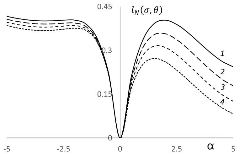
Normalized regrets for different variances the Bayesian risk is maximal. As an example, consider the approximate finding the minimax risk at K = 18, M = 1 on the set Ө = {(m, D) : 0,7 = D < D < 1 = D,m = a(D/N)1/2, |a| < 5}. In this case, approximately the worst-case prior distribution was found as Pr(D = 1,a = 1,9) = 0,3, Pr(D = 1,a = -2,2) = 0,15, Pr(D = 1,a = -5) = 0, 55, the corresponding Bayesian risk is approximately 0,41. Then, regrets were calculated for the strategy found. In Figure, lines 1, 2, 3, 4 correspond to regrets, calculated in increments of 0,5, at variance values of D = 1, 0, 9, 0, 8, 0, 7. One can see that the maximum values of the regret are approximately the same as the Bayesian risk calculated with respect to the worst-case prior distribution.

Conclusion

We obtained recursive equations for computing Bayesian risk and regret in the usual and invariant form which make it possible to compute them for any number of data multiples of the number of batches. To find minimax strategy and risk, one should determine them as Bayesian ones on the worst-case prior distribution.

research was supported by Russian Science Foundation, project number 23-21-00447,