
Inverse kinematics algorithm for trajectories with specified tool orientation
Журнал: Nanotechnologies in Construction: A Scientific Internet-Journal @nanobuild-en
Рубрика: System solutions for technological problems
Статья в выпуске: 5 Vol.18, 2026 года.
Бесплатный доступ
Introduction. During welding, coating application, and assembly or installation operations, the tool’s position is specified in conjunction with its orientation. A single specified pose may correspond to various sets of manipulator joint angles, and the solutions obtained for individual points do not always form a continuous trajectory. In such cases, the transition from one point to another involves a sudden change in joint angles, a factor that must be taken into account when setting movement speeds. The trajectory is defined either by joint angles or by an array of Cartesian tool poses. In the latter case, the input data consists of coordinates and orientations derived from a CAD model, teach points, or an external planner. Calculating the trajectory from this data requires reconciling inverse kinematics solutions at adjacent points; in the algorithm under consideration, this is achieved by passing the calculated angles to the computation for the next point. Methods and Materials. The object of study is a six-link manipulator with six degrees of freedom. Joint angles were determined based on specified Tool Center Point (TCP) positions and orientations using the pseudoinverse of the numerical Jacobian matrix, while the orientation error component was calculated using ZYX Euler angles. The solution obtained for a given point served as the initial approximation for the subsequent point. Verification was performed using trajectories comprising varying numbers of points. Results and Discussion. The procedure for formulating the six-dimensional error, the Jacobian calculation, and the iteration termination criteria are presented. Position and orientation errors, iteration counts, and computation times were determined for trajectories consisting of 5, 10, and 20 points; trajectories with up to 50 points were also examined. Calculation results for an identical geometric trajectory showed average iteration counts per point of 28, 18, and 12, respectively. Utilizing the previous solution reduced the number of iterations and, in the tests conducted, enabled the maintenance of the selected solution branch. Conclusion. The developed algorithm enables the derivation of a sequence of manipulator joint angles from a set of tool positions and orientations. In the calculations performed, the transfer of the solution between adjacent points ensured smooth angular variation; however, this mechanism alone does not guarantee the avoidance of a solution branch switch for every possible trajectory. The algorithm’s applicability is constrained by the convergence conditions of the numerical computation. When approaching a singular configuration or using sparse point spacing, it is necessary to additionally check the condition number of the Jacobian. Enhancing computational stability may require finer trajectory discretization and regularized pseudo-inversion.
Короткий адрес: https://sciup.org/142249022
IDS: 142249022 | DOI: 10.15828/2075-8545-2026-18-5-681-690
Текст научной статьи Inverse kinematics algorithm for trajectories with specified tool orientation
Original article
Кулаков П.А., Афанасенко В.Г. Алгоритм обратной кинематики для траекторий с заданной ориентацией инструмента. Нанотехнологии в строительстве. 2026;18(5):681–690. – EDN: BDBXER.
Controlling a manipulator along a trajectory requires specifying the tool’s position and orientation at each point. This approach is used in seam welding, coating application, assembly, and gripper positioning. For a single target pose, inverse kinematics yields one or more sets of joint angles. During continuous motion, it is necessary to select solutions that avoid configuration jumps and exceedance of permissible joint speeds [2–5].
Trajectory problems are solved in either joint space or cartesian space [2–4]. In the former case, joint angles are specified as functions of time, while the TCP position and orientation are determined via forward kinematics. In the latter case, a sequence of target poses is defined, and the inverse kinematics problem is solved for each pose.
Nanotechnologies in construction
Нанотехнологии в строительстве
2026; 18 (5): 681–690
Nanob
SYSTEM SOLUTIONS FOR TECHNOLOGICAL PROBLEMS
This approach is advantageous when the trajectory is derived from a CAD model, teach points, or data from an external planner. However, using an arbitrary initial guess can cause the algorithm to switch to a different solution branch. This results in discontinuities in the joint angle sequence, complicating time-based interpolation [3, 4, 11, 12]. In this study, the solution obtained for the previous point is used for the next point; with a sufficiently small step size, this technique preserves the selected solution branch [2–4].
The influence of the sampling step on the continuity of joint coordinates is discussed in [3, 4, 11–15]. When poses are specified at sparse intervals, the solution for a given point may not be sufficiently close to the solution for the subsequent point, causing the difference qi +1 – qi to increase. This constraint is particularly significant near singularities, during a switch between solution branches, and when there is a substantial change in tool orientation. Therefore, the step size between points is selected based on changes in position and orientation, rather than solely on the number of trajectory nodes. The initial trajectory is represented as an array of target poses obtained from teaching points or an external planner [3, 4, 11, 12].
The study utilized the kinematic model of the STP3 project [17], for which the forward kinematics, a numerical Jacobian, and an inverse kinematics algorithm for a single pose had previously been derived. The objective was to develop and validate a trajectory calculation algorithm based on specified TCP positions and orientations. The algorithm takes an array of target poses as input and generates a sequence of joint angles as output. To achieve this goal, continuity conditions were formulated, a method for specifying orientation was selected, convergence criteria were defined, and calculations were performed for 5, 10, 20, and 50 points.
A six-link manipulator is considered, the kinematics of which are defined by Denavit-Hartenberg parameters. The model corresponds to an anthropomorphic manipulator with revolute shoulder, elbow, and wrist joints. Parameter values are provided in [17]. Forward kinematics defines the mapping q → T06(q), where T06(q) is a 4×4 homogeneous matrix of the form [R(q) p(q); 0 1], q ∈ I6 is the vector of joint angles, p(q) ∈ 13 is the TCP position, and R(q) ∈ SO(3) is the tool orientation matrix [1–5, 17]. For a given pose Td = (Rd, pd), it is necessary to determine a vector q* satisfying the conditions ‖ p(q*) – pd ‖ ≤ εp and ρ(R(q*), Rd) ≤ εR. The quantity ρ(·,·) characterizes the orientation mismatch.
An array of positions pi ∈ R3 and an array of orientations Ri ∈ SO (3), i = 1, … , N are given. The objective is to determine a sequence of joint angles qi ∈ I6, i = 1, … , N , such that, for each i , the matrix T 0 6 ( qi ) corresponds to the specified pose Ti = ( Ri | pi ) within a prescribed tolerance. The differences ‖ qi +1 – qi ‖ between consecutive points must not result in exceeding permissible joint velocities and accelerations during time-based interpolation [2–4, 11, 12]. The initial guess for point i + 1 is set to the solution obtained for the previous point: q 0 ( i +1) = qi .
The orientation is defined by Euler angles in the ZYX convention, which are subsequently used to construct a six-dimensional error vector:
R = Rz ( ψ ) Ry ( θ ) Rx ( ϕ ), η = ( ϕ,θ,ψ ) T .
Taking into account the positional and orientational components, an error vector is obtained
P = (p
The first three components characterize the position error, while the last three characterize the orientation error [7–10]. This representation is used when constructing the numerical Jacobian. Special handling of the angles is required in the vicinity of gimbal lock.
It is assumed that the target poses are reachable and not located in the immediate vicinity of singular configurations. If this condition is violated, the Jacobian becomes ill-conditioned, the number of iterations increases, and a small change in the target pose can cause a significant change in the angles [5–9, 16]. Therefore, alongside solving the inverse problem, it is necessary to monitor the stability of the calculation and select an appropriate trajectory step size.
METHODS
The calculation is performed sequentially for points i = 1, … , N , with an internal iterative calculation carried out for each point. For i = 1, the initial approximation q 0 (1) is set as either the zero configuration or a known configuration close to the first target pose. For the remaining points – that is, for i ≥ 2 the previously obtained solution is used:
q0(i) = q*i–1, where the initial approximation is set equal to the result from the previous point. At iteration k, we first deter-
Nanotechnologies in construction 2026; 18 (5):
Нанотехнологии в строительстве 681–690
Nanob
SYSTEM SOLUTIONS FOR TECHNOLOGICAL PROBLEMS

mine the current pose T 0 6( qk ) and the error ek , then find the numerical Jacobian J ( qk ) and the increment
∆ q = J +( qk ) ek .
After determining the increment, the angles are refined using the formula qk+1 = qk + λ∆q.
The iterative calculation terminates when ‖ ek ‖ < ε or after the specified number of iterations N max is reached
[5–9, 16].
The ZYX Euler angles (ϕ, θ, ψ) required to calculate the orientation error are determined from the rotation matrix R ∈ SO(3). When writing
R = Rz ( ψ ) Ry ( θ ) Rx ( ϕ )
the inverse transformation can be performed using the formulas
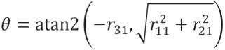
;
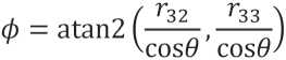
;
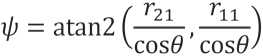
provided that cos θ ≠ 0 [9, 10]. Special handling is applied in the vicinity of gimbal lock, and the resulting angles are mapped to the interval [– π , π ]. These same angles are used in the six-dimensional error vector and in the calculation of the numerical Jacobian.
The Jacobian J ( q ) ∈ R6×6 relates the increment in angles ∆ q to the increment of the “position + orientation” state vector:
∆ x ≈ J ( q )∆ q .
The i -th column of the matrix is calculated using the finite difference.
f^ + Se^-f^q)
At each step, forward kinematics, error generation, Jacobian calculation, increment determination, and stopping criterion check are performed. In Figure 1 shows the sequence of operations and shows the transfer of the result of the previous point as an initial approximation.
The step size determines what fraction of the calculated increment is used to refine the angles. If the matrix J is well-conditioned, the increment is fully utilized when λ = 1; however, in the presence of a large initial mismatch, such a step may lead to oscillations in the solution. To limit the step size, values of λ ∈ [0.5, 1] are considered, or the coefficient is made dependent on the current error:
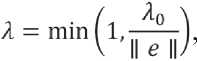
where λ 0 is the base coefficient for step-size selection [5–9]. A different approach was adopted for the calculations: a value of λ = 0.7 was selected based on preliminary

Fig. 1. Block diagram of the IK algorithm for the trajectory
Nanotechnologies in construction
Нанотехнологии в строительстве
2026; 18 (5): 681–690
Nanob
SYSTEM SOLUTIONS FOR TECHNOLOGICAL PROBLEMS
tests and used for all iterations. The relationship shown illustrates a possible method for varying λ ; however, adaptive step-size selection was not implemented in the version tested.
When formulating the error vector e ∈ В6, there are three positional components (expressed in meters) and three orientation components (expressed in radians). In the calculation model, these are included in the combined vector without additional weighting coefficients:

With this calculation, the overall norm depends on the chosen units for position and orientation. If the permissible orientation mismatch differs from the positional requirement, the influence of the angular component can be adjusted by introducing a weighting factor:
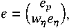
where wη ≈ 0.1 … 0.2 [7–10]. Separate tolerances can also be specified: εp for position and εη ≈ 10–4 rad for orientation, with wη = 1. In this case, the convergence condition is expressed as II г IK JfJ + f*. The error on the order of 10–8 rad observed in experiments allows for the use of separate criteria without imposing stricter requirements on the solver.
Figure 1 shows the data flow from the array of TCP poses to the array of joint angles. This scheme corresponds to the sequence of operations in the algorithm’s software implementation.
Calculations were performed in a Python 3 environment using the kinematic model described in [17]. The script `ik_trajectory.py` utilized functions for forward kinematics, the numerical Jacobian, and the inverse kinematics solution for a single pose. Coordinates were specified in meters, and angles in radians.
Three scenarios were considered. In the first case, the trajectory consisted of five points located along a straight line segment within the workspace; the tool orientation remained constant. In the second case, ten points were defined along an arc in the x – y plane at a constant height, with the orientation either remaining constant or changing to align with the direction of motion. The third scenario involved twenty points with a uniform change in position and a rotation of the orientation around the vertical axis.
For each scenario, the following parameters were determined: the number of iterations, the position error ‖ p ( qi ) – pi ‖, the orientation error based on the difference in Euler angles, and the total computation time for the sequence q 1 , … , qN [3–9, 11, 12]. Trajectory smoothness was evaluated based on the change in angles between adjacent points.
The calculations utilized a convergence threshold of ε = 10–6, a maximum iteration count of N max = 100, and a step coefficient of λ = 0.7. The value λ = 0.7 was selected based on preliminary tests; λ remained constant thereafter – meaning no adaptive step-size adjustment was applied. For the first point, the initial approximation was set to the zero configuration q 0 = (0,0,0,0,0,0), while the solution from the previous point was used for each subsequent point. No additional weighting factors for orientation error were introduced.
Calculations were performed on Windows 10 using Python 3.8 and the NumPy, SciPy, and Matplotlib libraries. The total trajectory computation time (excluding visualization) was measured using the time.perf_counter function. Based on the results, the TCP trajectory and plots showing position error and joint angle changes were generated.
Additionally, points at the boundary of the workspace and small pose variations relative to a previously obtained solution were tested. With small pose variations, the number of iterations decreased. Calculations were performed for a single geometric trajectory using N = 5, 10, 20, 50. As the number of nodes increased, the average number of iterations per point decreased. At N = 50, the total time was 1–2 seconds, making the algorithm suitable for offline planning.
For a trajectory consisting of 15 points, a 30° orientation rotation around the z -axis was specified. The resulting sequence qi was continuous, and the error did not exceed the established threshold. When the same extended segment was defined by only three points, a solution branch switch occurred in one of the calculations, resulting in a jump in joint angles. For trajectories of 10 and 20 points, the condition number cond( J ) remained within the range of 8–12. At certain nodes of the 5-point trajectory, however, it reached higher values. Consequently, the density of pose specification significantly influences the algorithm’s performance [2–4, 11, 12].
Nanotechnologies in construction
Нанотехнологии в строительстве
2026; 18 (5): 681–690
Nanob
SYSTEM SOLUTIONS FOR TECHNOLOGICAL PROBLEMS
RESULTS
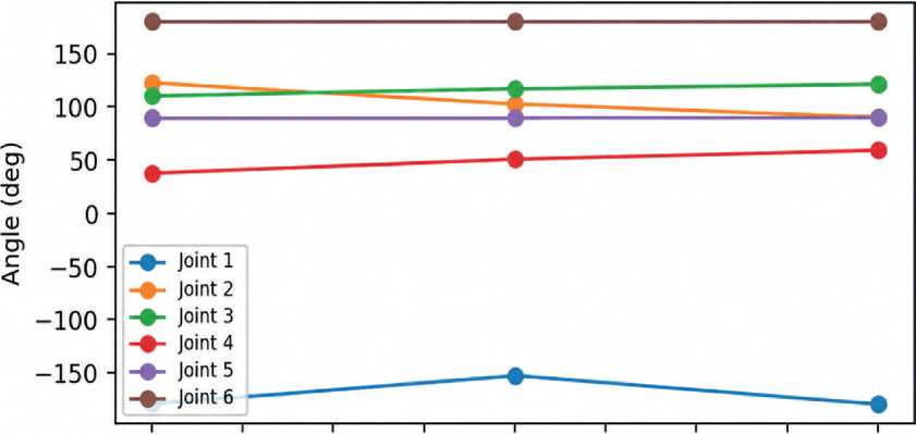
The convergence condition was met for five points. The highest number of iterations was required for the first point, for which the zero configuration was used. According to Table 1, the average number of iterations for this trajectory was also the highest. The position error did not exceed 10–7 m or 10–4 mm (Fig. 2). The resulting TCP trajectory matches the target trajectory within the specified accuracy, and the joint angles vary smoothly [5–10] (Fig. 3).
As the number of points increased, the average number of iterations decreased from 28 at N = 5 to 18 at N = 10 and to 12 at N = 20 (Table 1). Position and orientation errors did not exceed the specified threshold. The computation time for 20 points allows the algorithm to be used for offline planning (Fig. 4). Operation at a frequency of 100–500 Hz would require an analytical Jacobian or
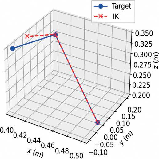
Fig. 2. Target and actual TCP trajectory in 3D (5 points)
0.00 0.25 0.50 0.75 1.00 1.25 1.50 1.75 2.00Point index
Fig. 3. Joint angles based on trajectory points
Nanotechnologies in construction
Нанотехнологии в строительстве
2026; 18 (5): 681–690
SYSTEM SOLUTIONS FOR TECHNOLOGICAL PROBLEMS
Nanob
Table 1. Number of iterations and inverse kinematics computation time for the trajectory
|
N points |
Average number of iterations per point |
Max. iterations per point |
Total time (ms) |
|
5 |
28 |
45 |
180 |
|
10 |
18 |
35 |
220 |
|
20 |
12 |
28 |
320 |
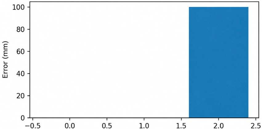
Fig. 4. Positioning error along trajectory points (mm)
Point index a faster implementation of the computational operations [3–8, 14–16].
For a trajectory consisting of 10 points, the position error did not exceed 10–7 m or 10–4 mm. This value is smaller than the relevant manufacturing tolerances; therefore, in practical application, accuracy will be determined by the kinematic model, calibration, and specified tolerances.
A comparison was made with a calculation in which a zero initial guess was specified for each point (Fig. 5). In that case, the number of iterations increased, and a switch to a different solution branch could occur. Using the previous result reduced the average number of iterations by a factor of 2–3 and eliminated discontinuities in the trajectories under consideration (Table 1). Thus, the initial guess affects both the computation time and the continuity of joint coordinates [2–4, 7–9].
The number of iterations and the computation time for a single geometric trajectory were compared across different discretization levels (Table 1). As N increases, adjacent target poses become closer to one another; consequently, the previously found solution requires fewer refinements when transitioning to the next point.
Table 1 shows that the average time per point decreases from 36 ms for a 5-point trajectory to 16 ms for a 20-point trajectory. At the same time, the total computation time increases from 180 to 320 ms: the reduction in the number of iterations per point does not compensate for the increase in the number of points themselves.
Nanotechnologies in construction
Нанотехнологии в строительстве
2026; 18 (5): 681–690
Nanob
SYSTEM SOLUTIONS FOR TECHNOLOGICAL PROBLEMS
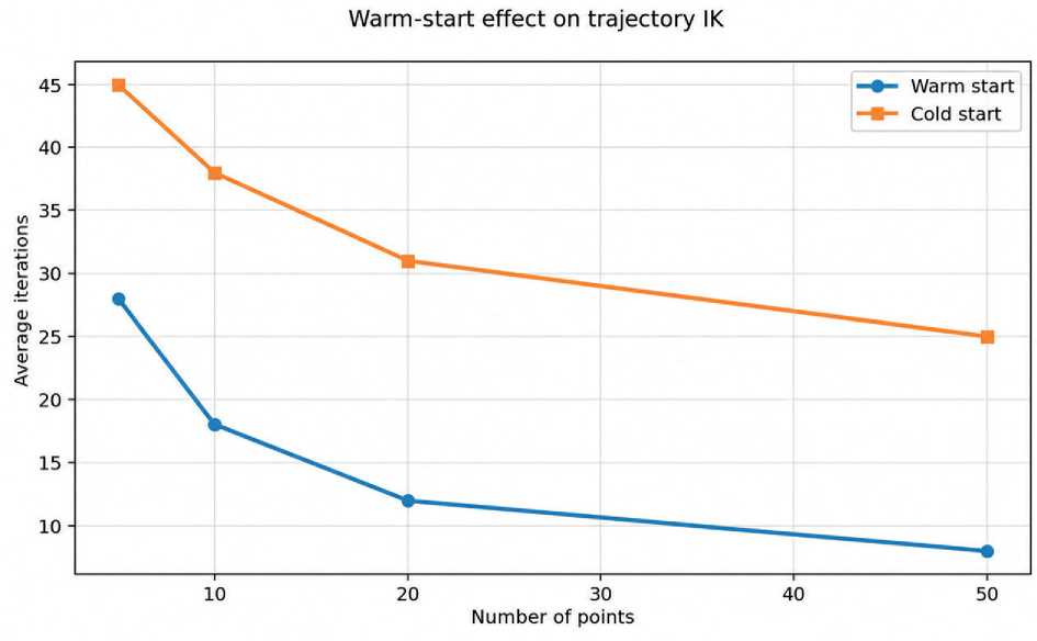
Fig. 5. Comparison of warm start and zero-order approximation
Table 2. Russian and foreign views on trajectory inverse kinematics
|
Criterion |
Russian practice |
International practice |
|
Primary focus |
Solution continuity and engineering resilience |
Warm start, branch consistency, task-space pipelines |
|
Representation of orientation |
More often Euler angles and matrix description |
Euler, quaternion, axis-angle |
|
Primary risk |
Switch solution branch |
Loss of continuity near singularity |
|
Typical sources |
Robotics training courses and engineering manuals |
Craig, Siciliano, Buss, Wampler |
CONCLUSION
Convergence conditions deteriorate as the system approaches a singular configuration; furthermore, if poses are defined sparsely, a switch in the solution branch may occur even when using the previous result. For trajectories consisting of 10 and 20 points, the condition number remained moderate, whereas an increase was observed at specific nodes of a 5-point trajectory. These results highlight the need to monitor cond(J), refine the discretization step, and apply regularization when signs of instability arise [7–9, 16].
The algorithm enables the determination of joint coordinates based on Cartesian poses specified by an operator or a CAD system, thereby reducing the manual effort required for trajectory definition. Future research could focus on incorporating joint constraints, avoiding singular configurations, utilizing an analytical Jacobian, and validating the algorithm on a physical manipulator [3, 4, 11–17].
Nanotechnologies in construction Нанотехнологии в строительстве
2026; 18 (5): 681–690
SYSTEM SOLUTIONS FOR TECHNOLOGICAL PROBLEMS