Inverse Problem of Recovering Fluxes from Integral Data

We examine the parabolic system of the form

Mu = ut — Lu = f (x, t), (x,t) € Q = G x (0, T), where Lu = ^^=1 djaijuxi — ^П=1 aiuxi - aou, G C Rn is a bounded domain with boundary Г, aij, ai are matrices of dimension h x h. The equation (1) is furnished with the initial-boundary conditions

Ru|s = g, u(x, 0) = uo(x),(2)

where Ru = ^^ =1 a ij (t,x)v jdu + a(x,t)u (v is the unit outward normal to Г, and the overdetermination conditions

У (u(t,x),(pi (x)) dx = ^i (t), i = 1, 2,...,m,(3)

G where the brackets (•, •) stands for the inner product in Rh and ^j are linearly independent vectorfunctions. The function g in (2) is of the form g = i=1=1 ai(t)Ф(t,x), where the functions ai are to be determined and {Фi} are known linearly independent vector-functions. The problem is to find a solution u to the equation (1) satisfying the conditions (2), (3) and the functions {ai(t)}.

Inverse problems on determining boundary regimes arise in many of areas of mathematical physics, in particular, when modeling heat transfer processes and designing heat-protective materials, modeling the properties and thermal regimes of composite materials, modeling the thermal regimes of soils in the permafrost zone, in environmental problems (see [1–3]). The most used additional conditions are temperature measurements at some collection of points lying inside the domain or on its boundary. These problems are well-posed only in the latter case and the existence and uniqueness theorems in inverse problems of recovering the fluxes or the heat transfer coefficients with pointwise measurements are exposed in [6, 7]. The problem of recovering fluxes with arbitrary location of the measurements points is considered in [8], where the uniqueness and existence theorem was obtained under rather rigid constraints on the data. Note also the articles [9, 10], where in the model case the uniqueness theorem of a classical solution to the problem of recovering of the heat transfer coefficient a(t) was obtained with the use of both the pointwise condition u(t, xo) = a(t) and the integral condition of the form (3). Pointwise conditions are also employed in [11] in the case of n = 1. In the articles [12,13] the integral conditions of the form (3) are used as some approximation of the pointwise conditions. The problems (1) – (3) are considered in [14,15], in the former of them some model problem was examined with g = g(t), the latter contains more general results but for a single equation. In contrast to other results, we consider inverse problem for a system of equations and our conditions for the data are a much weaker than those in [15]. Moreover, the overdetermination conditions are actually do not assume that they are valid for all components of a solution. It is possible that some of them do not occur in (3). The article is devoted to well-posedness of the problem (1) – (3). Under certain conditions it is proven that there exists a unique solution to the problem from some Sobolev space. We also describe a numerical algorithm and the results of numerical calculations.

1.    Preliminaries

Let E be a Banach space. The notations for Sobolev spaces W pS ( G ; E ), W s (Q; E), etc. are standard (see [17,18]). If E = R or E = R ⁿ then we denote the last space simply by W pS ( Q ). Definitions of Holder spaces C ^a,e (Q),C ^a,e ( S ) can be found, for example, in [19]. By the norm of a vector, we mean the sum of the norms of coordinates. Given an interval J = (0 , T ), denote W S ^,r (Q) = W ^s (J ; L p ( G )) П L _P (J ; W p ( G )). Similarly, W p ^,r (S ) = W ^s (J ; L p (r)) П L p (J ; W r (Г)). Let (u,v) = f ( u(x),v(x) ) dx. All considered spaces and coefficients of equation (1) are assumed

G to be real. Next, we assume that Г G C2 (see the definition in [19, Chapter 1]). Introduce the notations Qy = (0, y) x G and Sy = (0, y) x dG.

The space W _p ^s (0 , в; E) ( s G (0 , 1), E is a Banach space) is endowed with the norm ll ? ( t ) ll w«(o ,0 ; E ) = ( ll< _p (0 ,e ; E ) + <  q ^p)^ , <  q > p= f в ^-2^d^ • If E = C then we obtain the usual space W pS (0 ,e )• For s G (0 , 1), let W ps (0,e; E') = { q G W pS (0 , в ; E ) : t ^-s q(t) G L p ^(0,e; ^{E ) }} . It is a Banach space with the norm ^l q^{(t) l} W s (₀ , _{в ; Е} ) = II q IlL p ( ₀ ,_{e ; E} ) + <  q > ^p p . ^For s >  1 /p , all functions q from this spaces possess the property q(a) = 0 and, for s = 1 /p , the above norm and the usual norm in || • ||w _js (0 ,e _; E ) are equivalent for the functions q(t) such that q (0) =0 if s >  1 /p (see Lemma 1 in Sect. 3.2.6 [16]). The spaces W _p (0,e ; L _p ( G )), Wps^^Q e ) = W pS (0,e ; L _p ( G )) ^ L _p (0,e; W _p ^{2 s} ( G )), for s = 1/p, include functions v(t,x) in W pS (0,e ; L _p (G)) and Wp ’ ² s ( Q _a ), respectively, such that v (0 ,x ) = 0 whenever s >  1 /p . The norms H • H w s, 2 s ( Q e ) , H • H w s (o e ; L ( G )) are defined with the use of the above norm in W pS (0 , в ; E) and we have

β             ββ

=         dux ₊ / / / M/MMMlp..   _{+ H} ^p

Wp ( Q _e )     J J      t ^s p             J J J      | t - _T | ¹⁺ sp                      L p ^(0,e ; ^WP^(G))

G 0                    G 0 0

The spaces W _p (a,e ; L p (Г)) and W_p ^,2s (S e ) are defined by analogy.

Lemma 1. Assume that s G (0 , 1) , s = 1/p and p G (1 , от ) . Then

• 1)    the product q • v of functions q G Wp (0 , т ) , v G W< s 0 ^2s (S _T ) П L _p (r; L ^ (0,t )) ( q 0 = p if s > 1/p and q 0 > 1/s if s < 1/p) belongs to W_p ^,2s (S _T ) and we have the estimates

^{H q}v ^H W s (0 ,T ) ^- c 1 ^{H q H} W s (0 ,T ) ^{( HvH} W _q ^s ₀ (0 ,T ) ⁺ v L ,. (0 ,T ) ) a.a. ^{on Г} ,

^{H q}v ^H W s’^{2 s} ( S ) - c 2 ^{H q H} W _p ^s (0 ,T ) ^{( H} v ^H W _q ^s ₀ ^{2 s} ( S ) ^{+ H} v ^H L p (F; L ^ (0 ,T )) ^{); (4)}

if q(t) G WpS(0,T) (т G (0,T]) and v(t,x) G W®2s(S) A L^Qr) then qv G Wp2s(ST) and h^Ws(0,T) - c3llqllws(0,T)(Hvllws,(0,T) + llvHL_(0,T)) - Mqllws(0^)HvHWqS0(0,T) a.a. on Г,

• ^Hq v ^H WW/ ^,2s ( S T ) ^- c ^{5 HqH} W _p ^s (0 ,T ) ^{( HvH} W _q ^s 0 ^2s (S t ) ^{+ H} v ^H L p (F;L ^ (0,t )) ) ^- Mqllw s (0 ,T ) ^HvH W _q ^s 0 ^2s ( S ) , ⁽⁵⁾

where the constants C 3 — c g are independent of q,v and т G (0 , T ] . The claim of the lemma remains valid if we replace Г , S with G, Q .

Proof. The proof in the case of s >  1 /p is exposed in Lemma 1 in [15]. Similar arguments can be used to treat the case of s <  1 /p . So we omit the arguments.

□

Fix so = 1/2 — 1/2p and assume that aij G C([0,T]; W.(G)) П L . G; Ws^(0,T)), a G W 2(S) П L. (Г; W(0,T))

(( n + 1) / 2 q 1 <  1 — 1 / 2 p ) , а ^ | s G W^ ² * ⁰ ( S ) (( n + 1) / 2 q 2 < s o ); (6)

ai G L.(G; W. (0,T)) П Lq3 (Q), q3 > (n + 2), (i = 1,...,n), ao G L.(G; Wsq°0 (0,T)) П Lq4(Q), q4 > (n + 2)/2, (7)

where i,j = 1 , 2 ,..., n , q o = p if p >  3 and q o >  1 /s o if p <  3.

State the Lopatinskiy and parabolicity conditions. Consider the map A o ( t, x,£ ) = £П . = ₌ | a ij (t,x)^ i £ j and assume that

^Фа G [0,n/2) : a(Ao(t,x,£)) С SфA = {z G C : |argz| < Фа}(8)

for all £ G R ⁿ with ||£|| = 1 and ( t,x ) G Q. Put B o u = ^ n.j₌₁ a ij V j u x i . The Lopatinskii condition is written as: given an arbitrary point ( t o ,x o ) G S , the boundary value problem

(A + Ao(to,xo,£ + v(xo)dz)v(z) = 0, Bo(to,xo,£ + v(xo)dz)v(0) = hj, z G R+, has a unique solution from C(R+; E) vanishing at infinity for all £ G Rn, A G Sп-фA, and hj G E such that £ • v(xo) = 0 (v(xo) is the unit exterior normal to Г at xo) and |£| + |A| = 0.

Conditions on the data:

f G Lp(Q), uo(x) G W2-2/p(G), p = 3;(10)

g G WS°,2s°(S), g(0,x)|r = B(0,x)uo|r if p> 3;(11)

^k G W^(G), Фк G W^’2*0(S), ^k G Wpo+1(0,T), (f,^k) G Wp(0,T), where qo = p if p > 3 and qo > 1/so if p < 3, k = 1, 2,... , m, and p‘ = p/(p —

Theorem 1. Let G be a bounded domain with boundary of the class C ² and let the conditions

• (6 ) - (11) hold, where p = 3 . Then there exists a unique solution u to the problem (1)-(2) such that u G W p (Q). A solution satisfies the estimate

H u ll WA ² ( Q ) - C f ^ L p ( Q ) ^{+ l} u o ^l _W 2 - ²/ ^p ( _G ) ^{+ l g l} W _i 1 /² - ¹/²P’¹ - ¹/p ( _S )) .

Existence and uniqueness of solutions to the problem (1), (2) results from the known results on solvability of parabolic problems (Theorem 2.1 in [17, 21] or Theorem 5.3 in [22]).

Theorem 1 validates the following statement.

Theorem 2. Let G be a bounded domain with boundary of the class C ² and let the conditions (6) - (11) hold, where f = 0 and u o = 0 , p = 3 , g G W j} /² ^p, ^{1 1/p} (S ) . Then a solution u G Wp ’ 2 (Q)

to the problem (1), (2) meets the estimate | u | w i , 2 ( q ) — c | g | c is independent of y G (0 , T ] and g .

˜

W_p i / ₂ - / ₂ p, i - i /p

, where the constant ( S Y )

Proof. The proof coincides with that in [15, Theorem 2].

□

2.    Main Results

In addition to the conditions of the previous section, we require that

| det B ( t ) | >  S o >  0 V t G [0 , T ] , У ( u o ( x~ ),V k ( x ) ) dx = 0 k (0) , k = 1,...,m,       (13)

G where B(t) is the matrix with entries bij = f ^i(x)^j(t,x) dr;

г

• (A) if p >  3 then the function B(0,x)u o ( x ) | r belongs to the linear span of the functions Ф 1 (0 ,х ) ,... , Ф т (0 ,х ).

The main results of the article is the following theorem.

Theorem 3. Assume that G is a bounded domain with boundary of the class C 2 , p = 3 , and the conditions (6) - (10), (12), (13) , (A) hold. Then there exists a unique solution (u,q) (q = (q i ,... ,q m )) to the problem (1) — (3) such that u G W p, (Q), q G W s ⁰ (0,T) . A solution meets the estimate

^u^Wp’2(Q) + 11^11 wpS0(o,T) - m

- C (Il f Ik. ( Q ) + 1Ы1 2 - 2 , +        ll w ;+. (0 ,T ) + IKf.W«W?(0 ,T ))) .

^W p   ^{( G )}    i =1         ^p

Proof. First, we consider the case of p >  3. In this case, the condition A) holds and thus there exists constants q i (0) such that B(0,x)u o | г = Sm ti q i (0)Ф i (0 , x ). In view of (13) these constants are determined uniquely. The conditions (12) and Lemma 1 imply that if q G W ^s 0 (0,T ) then q i (t)Ф _i (t,x) G Wp ⁰ ’ ^{2 5 0} ( S ) and, respectively, g G Wp ⁰ ’ ^{2 5 0} ( S ). In particular, ^ 0 =1 q i (0)Ф _i (t,x) = g o (t,x) G W p ^{0 ,2s} 0 (S ). Let v G W p^{, 2} ( Q ) be a solution to the problem (see Theorem 1)

Mv = f, Bv l s = g o (t,x), v\ t =0 = u o (x). (14)

Make the change of variables u = v + w . In this case the function w G W_p ^{1 , 2} ( Q ) is a solution to the problem

Mw = 0 , Bw \ s = g - g o = g, w \ t =o = 0 .                       (15)

The condition (3) can be rewritten in the form

У ( w,^ k (x) dx = 0 k

G

У ( v(t,x),^ k (x) ) dx = ^ k , k = 1 , 2 ,...,m.

G

In view of (13), 0 k (0) = 0 and, as is easily seen, 0 k (t) G W p (0 ,T ). Below we shall demonstrate that 0 k (t) G W ^+ s ⁰ (0,T ). Multiply the equation in (15) scalarly by ^ k (x) and integrate over G . We obtain that (w t ,^ k ) = (Lw,^ k ). If ( u , q) is a solution to the problem (1) - (3) then integrating by parts and (15), (16) yield

m

0 ' k ^{( t )} =

(aw, ^k) dr + ^ qi(t) / (Фi, ^k) dr, г                 i=1      г qi(t) = qi(t) - qi(0),

where k = 1 ,..., m and a(w, ^ k ) = — f Y nj ₌₁ { a ij w x i ,r kx j ) — 0 ^ 0 =1 a i w x i + a o w, V k ) dx. The

G last equality can be rewritten in the form

m

^ q i (t) / ( Ф i , ^ k ) dr = -0 k ( t ) - a(w, V k ) + I ( aw, ^ k ) dr, i ⁼ⁱ       г                                     г

or in the form

Bg a = F, F = ( F 1 ,...,F r ) ^T , F k

= ^^k( t ) - a(w,^ k ) + У ^w^ k dr, г

where qa = (q1,... ,qm)T. The function w in (18) is a solution to the direct problem (15). The entries bij of the matrix B are such that bij G Ws0(0, T) and, furthermore, llbij IWO (0,T) — H$j HLq0 (r;Ws0 (0,T)) bi ^Lq‘ (Г), q‘ = q0/(q0 — 1), where the parameter q0 is that of the condition (12). Similarly, llbij IIl~ (0,T) — ll^j Hl^ (0,T;Lp (Г)) ll^i ^Lp‘ (Г) — ch^j ILp (Г;£„ (0,T)), p = p/(p - 1),

By Lemma 1, the products of any number of the entries bij belongs to Wqs00 (0, T) and thus the entries of the matrix B—1 also possess this property. The condition (13) yields qa = B-1F = R(qa)= g + R0(qq),(21)

where g = B ^{— 1 g} , ^g = (Ф 1 , Ф ₂ ,..., ^ r ) ^T , ^ k ( t ) = b k ( t ). Next, we prove that this equation is solvable, at least on some small time interval. Consider the segment [0 ,5 ] C [0 , T ]. Estimate l|R0 ( q a )ll w s o (o ,5 ) ■ By Lemma 1, we infer

^H R ^{0 ( q} a ^{) H} W s^o (0 ,5 )

m

^— c ^^{( H} a^(w,r k ^{) H} W s o (0 ,5 ) k =1

+

"/

Г

^w^k > 5Г|^о (0 ,5 )

) .

By definition,

a(w,^p k )

-

n

J 12 ( a ij w x i

G i,j =1

n

,pkx ) + (£ i=1

a i W x i + a 0 w),^p k ) dx.

The Minkowki and H¨older inequalities and Lemma 1 yield

J =

"/

G

^{( a} ij w x i , ^p kx j ) ^dx II w s 0 (0 ,5 )

^— c ¹ (y ^H^ w ^H W s o ( ₀ ,₅ ) ^dx) p ^— c ¹ llwll w S⁰ (0 ,5 ; W 1 ( G )) .

G

If w is the zero extension of w to the interval (-№,5) then it is easy to check that the norms ||w||wso(0 5-W1(G)) and ||w||wso(-M5-wi(G)) are equivalent with constants independent of 5. The definition of the norm and [18, Theorems 4.1.3, 4.5.5 of Ch. 7] yield llwllwS0(0,5;W1 (G)) — cblwlW0(-^,5;W1(G)) — c25Y0 IMW0^0(-^ ,5;Wp1(G)) — c35Y0 IMhso+Yo+^°(—^,5;Wp1(G)) — c45Y0 llwllw1’2(Q^) — c45Y0 HwHW1’2(Qs), (24)

where 0 < Y 0 <  1 / ² — S 0 — ^£ 0 , ^£ 0 >  0, and Q ^ = ( -№ ,5 ) x G . The relation (24) validates the estimate

^H У ( a ij w x j ,^p kx i )^dx|l w s ⁰ (0 ,5 ) ^{— c} 6 ⁵ Y ^{0 H} w ^H w p i ’ ² ( Q _S ) ,                         ⁽²⁵⁾

G where the constant C6 is independent of 5. The summands I1 = ((awwxi,^k) dx and I2 = f (a0w,^k) dx in a(w,^k) are estimated by analogy and the estimates are simpler. So we omit G them. Proceed with the last summand J1 = || J(cw, Gk) dr||wso(0 5). We have (see (24)) that

J ^{1 —} c ¹ llwll w S⁰ (0 ,5 ; L p (Г)) ^— c bl wll Wp ⁰ (0 ,5 ; W 1 ( G )) ^— c ^{3 5 Y 0} llwll W p1’ ² ( Q _s ) .               ⁽²⁶⁾

Here we have used the embedding W p 1 ( G ) C L _p (r) and the Holder inequality. The estimates (25), (26) and the corresponding estimates for I i ,l 2 imply that

I|R№)IIwso(0,.) < c^Y0IMW1,2(Q.), where the constant C4 is independent of 5. Theorem 2 yields

|w|w1,2(Qi) < cHgHw;0i2s0(ss)•

By Lemma 1, ||g|| w s ₀ , 2 s ₀ (s ) <  c i £” =! H q i Hw^s 0 (0 5^ Here the constant c i depends on the norms ||Ф i l w s ₀ , 2 s ₀ (s) . In this case it follows from (27), (28) that

m

HR0(qa) llws0 (0,5) < c55Y0 £ llqillwso(0,5) = c55Y0 llqallwso(0,5), i=i where the constant C5 is independent of 5 and qa. Thereby, if 5J0C5 < 1 then the operator R0 is a contraction and, by the fixed point theorem, the equation (21) has a unique solution from the space WpS0 (0,50) under the condition that ^k G Ws0 (0, T). In view of the conditions of the theorem ^k G WpS0(0,T). Demonstrate that ^0k = / v(t,x)^k(x) dx G Wp+s0(0,T), i. e.,

G f vt(t,x)^k(x) dx G Ws0(0,T). Multiply the equation in (14) by ^k and integrate the result over G

G . We obtain that

m av^k dr + £t/i(0) / ^i^k dr + (f,^k), k = 1,...,m.     (30)

г               ^{i =1}       г

Repeating the arguments used in the proof of the estimate for H Rq allw ^s 0 (0 5 ) , with 5 = T , we can show that the right-hand side in the above equality belongs to W s ⁰ (0,T ) and, thus, Rk G Wp ⁺ s ⁰ (0 , T )• We have proven that the equation (21) has a unique solution (in correspondiong ball) on the segment [0 ,5 0 ]. Next, we can define a solution w G Wp ^{, 2} ( Q 5 ₀ ) to the problem (15). Demonstrate that the conditions (16) hold. Multiply the equation in (15) by ϕ _k and integrate over G . Integrating by parts and the estimates (14), (15) imply that

У { w _t ,^ k > dx

G

m

{ aw,^ k > d r + ^t[ i ( t ) / ( Ф i ,^ k > d r , k = 1 ,...,m.

г                   ^{i =1} г

The vector-function q^ _a meets the system (17), summing its k th equation with the equality obtained, we derive that j { w _t , ^ k > dx = ^ k , k = 1 , • • •, m. Integrating this equality with respect G

to t and using the initial condition, we justify (16) on [0 ,5 0 ]. Next, we show that a solution is extendible to the whole segment [0 , T ]. We have defined the vector-function q a only on [0 ,5 0 ].

Extend the vector-function q a by zero for t <  0 and assign q b =

{

q _a (t), t G (0 ,5 0 ) ^q a ⁽²⁵ 0 ^— t), t ^{G [ 5} 0 ^{,T ]}

Denote

by q 1 , • • •, q b the coordinates of the vector q b. The new vector-function q b belongs to Wp ^{0 , 2 s} 0 ( S ). Make the change of variables q ¹ = qq — q b . This vector-function with the coordinates q^ satisfies the system of equations

m

£ qi^(t)b ki = ^r k ^{( t ) — a(w,}V k ) + / (^aw , i =i                                  _г

m

^ k > d r — £ q i (t)b ki • i =i

In view of the definition, the vector q ¹ vanishes on [0 , 5 o ]. Let w o be a solution to the problem Lw o = 0 , Bw o | s = £™ i q^ i , w o | _t =o = 0 . In this case the function w i = w — w o is a solution to the problem

m

Lw i = 0 , Bw i | s = £ q 1 $ * >w i | t =o = 0 .                       (31)

i =1

By Theorem 1, w i =0 for t G [0 , 5 o ]. Thus, the extension problem for the function q a is reduced to determining a solution to the system

m

£ Q^b ki = ^ 1 k ^{( t )}

i =1

—

a ( w i ,^ _k ) +

У aw i ^ k dr,

Γ

where ^ik = ^'k(t)-a(wo, ^k) + f {awo, ^k) dr — £™1 qi(t)bki, and the function w1 is a solution to Γ the problem (31). This soluton vanishes for t < 5g. We have obtained the same system as before, but the Cauchy data are given at t = 5 and the right-hand side of the system (more exactly the vector ^g) differs from the previous one. Next, we can repeat the arguments of the previous proof on the segment [5o, 25o]. They are the same and without loss of generality we can assume that the constants arising in the proof of the estimate for the norm of the operator R0 are the same. Thus the system (32) is solvable on the segment [5o, 25o]. Repeating the arguments on [25o, 35o], etc. we construct a solution on the whole segment [0, T]. The estimate from the statement of the theorem was actually obtained in the proof of the theorem. Consider the case of p < 3. Take go = 0 in (14) and g = g in (15). Next, we repeat the arguments without any distinctions.

□

3.    Numerical Algorithm

The numerical algorithm employs the idea of the proof of Theorem 3. The equation under consideration is as follows:

Mu = u _t — Lu = u _t — div(c(x, t) V u) + b ( x, t ) V u + a ( x, t ) u = f, ^b(x, t ) = ^{( b} 1 ^{( x} , t),..., b n ⁽ x, ^{t)) T} , ^V u =⁽ dX i ,..., du n ^{) T} , ⁿ = ^{2, 3} ,

where ( t, x ) G Q = (0 , T ) x G and c is a diagonal matrix. Below we consider the case of n = 2 and assume that G = (0 , X ) x (0 , Z ), ( X, Z >  0). As before, Г = dG , let F o = { ( x 1 , 0) : X 1 G (0 , X ) } , S = (0 ,T ) x Г, S o = (0 ,T ) x F o . The additional measurements and the initial and boundary conditions are of the form

У u(y, t)^ i ( x ) dx = ^ i (t), i = 1 , 2 ,... , r,

G u|t=o = uo(x), c2ux2|so = g(t,x), u|s\So =0, or dN + au|s\so = °-           (35)

We employ the method of finite elements (FEM). The unknown function g is sought in the form g = ^1a j a j ( t )^ j ( x 1 ), where the functions a i are unknowns. We assume that

X

Bo — det ^{ b ij ^} , b ij —

У Ф j ( x 1 )Ф i ( x 1 , 0) dx 1 , 0

detB o = 0 .

Given a triangulation of G and the corresponding basis { ^ i }^ 1 which is defined in accord with the choice of the boundary conditions in (35). Denote the nodes of the mesh by { b i } . An approximate solution is sought in the form v = ^i=1 C i (t)^ i . The functions C i are determined from the system

MC t + K ( t ) C = — F + f, C = ( C 1 , C 2 ,..., C _N ) ^t , i = 0 , 1 , 2,...,N,          (36)

where XX F = (/ 9(t,xi )^i(xi, 0) dxi ,---,j g(t,xi)^N (xi, 0) dxi )T, f = (fi,...,fr)T, fi = j f (t,x№i (x) dx.

G

The matrix M and K have the entries m ij = (^ i , ^ j ) = f ^ i (x)^ j ( x ) dx,

G

K jk = (c i (t,x)^ kx i ,^ jx i ) + (c 2 (t,x)^ kx 2 ,^ jx ₂ ) + (b(t,x) V ^ k ,^ j ) + (a^x^ k ,^ j ) .      (37)

If we consider the Robin boundary condition on S \ S q then to the above summands we need to add the quantity f a^ k щ d r. We have that C (0) = C q = ( u q ( b i ) ,... ,u o (b N )).

S \ S o

A solution to the system (36) is sought by the method of finite differences. Let т = T/M is time step. We replace the equation (36) with the system

-Ф           —

M C ^{i +i —} C i + K i +i C i +i = — F _{i +1} + f i +i , C i = {C1,...,C N ) ^T ,i = 0 , 1 ,...,M - 1 ,    (38)

т where Ck ^ Ck(ri), Fi ^ F(ri), fi = f(Ti), Ki = K(ri).

Introduce the following notations: $ (t) = ( ^ i ( t ) ,^ ₂ ( t ) ,...,^ _r (t)) ^T , $ i = $ (ri'), $ k = $ k (ri), a i = ( a ¹ ,.. .,a r ) ^T , a i ^ a (ri'), a k ^ a k (ir ), Ф k = ($ k (b i ),$ k (b 2 ) .. . ,$ k (b N )) ^T .

The analog of the overdetermination conditions (34) is the equalities ( MC i , Ф k > = $ k , where the brackets stand for the inner product in R N . The initial data are as follows: C Q = u o (b k ) for k = 1,...,N .

The vector Fi can be written in the form Aai, where the entries of A are as follows: alj = XX f Фj(xi)^i(xi, 0) dxi or Fi = £j=i Фaj, with ek = f Фj(xi)^k(xi, 0) dxi. qq

The system (38) can be written in the form

Ri+iCi+i = -rFi+i + rfi+i + mCi, 1 = 0, 1, 2,...,M — 1, where Ri+i = M + rKi+i. Inverting the matrix Ri+i and applying M, we infer

MCi+i = —rM (Ri+i)-1Fi+i + M (Ri+i)-i (rfi+i + MCi) i = 0,1, 2,...,M — 1,

Multiply the system (40) scalarly by Ф k . We obtain that

$+ = —r(M(Ri+i)-iFi+i, Фk> + (M(Ri+i)-1 (rfi+i + MCi), Фk>.

If e j are the columns of A , F i +i = ^ j ₌i e / a i +i , then this system can be written in a matrix form. Let the matrix B i +i has the entries b ki = ( M(R i +i ) ^-i e i , Ф k > . In this case the system (41) is rewritten as follows:

$i+i + Hi+i = —rBi+iai+i, H^+i = —(M(Ri+i)-i(rfi+i + MCi), ^k>.(42)

Decribe the sequence of the calculations. First, we determine the initial data C k = u o (b k ). Assume that we have calculated a i , C i . The vector a i +i is defined from (42). Inserting it in (38), we can find C i +i .

4.    Programm Realisation

In this section we present the results of numerical experiments. To determine the accuracy of calculations, we take given functions c , ^{^} b , a , f and the function g depending on the known functions Φ i and α i . By solving the direct problem (33), (35) we can find a solution u of this problem and thereby find the values (34). Next, using the data of the direct problem and overdetermination conditions, we can solve the inverse problem (33) – (35), and find the solution u and the functions α i . By comparing the original functions α i , u and the results of calculation, one can evaluate the convergence of the algorithm.

The characteristics of the computer are as follows: Processor: Intel(R) Xeon(R) CPU E5-2678 v3 @ 2.50GHz (2 two processors); RAM: 64.0 GB; OS: Windows 10 Pro x64.

We will use a rectangle with vertices (0; 0), (2 , 0), (2; 1), and (0 , 1) as the domain G . Let’s create a mesh using Delaunay triangulation. We employ four grids Z 1 = 103, Z 2 = 379, Z 3 = 1453 and Z 4 = 5689. Having obtained the coordinates of the grid nodes, it is possible to calculate arrays for known input functions (using symbolic computing software packages). Also we define the arrays of the nodes on sides of the rectangle where y = 0 and x = 0, x = 2. Note that we use the homogeneous Dirichlet condition on all side except for the lower side of the rectangle.

Let the time step be equal to τ = T/m , with m = 100. The next step is constructing the functions ^ i : we take the solution of the direct problem C dp and define ^ k = ( M • C d ³ ,Ф k ) ( k = 1 , 2 , . . . , r ; i = 1 , 2 , . . . , m ) as described in (34). We can also add random noise to a solution to the direct problem U d . Noise is represented as a random variable with the range n s G ( - 5 ; 5 ), where 5 is the percentage deviation. The resulting function is of the form ^(jT ) = (M • Cd’ • (1 + n s (jT ) / 100) ,Ф i ) . Introduce some quantities: the equality E _a = max i (max j | a ^j (iT ) — a ^j | ) defines the calculation error for the functions α i (the numbers α _i ^j are the result of calculations, a j ~ a ^j ( Ti ), j = 1 , 2 ,... , r ); the error of calculations of a solution C i,j to the inverse problem is defined as E _u = max i,j | C dp — C ij | , where i = 1 , 2,... ,N and j = 1 , 2 ,..., m ; T_T is the execution time of the algorithm in seconds.

For the first group of the data, we take coefficients of the equation: a = 1 / ( t + 1), b 1 = 0, b 2 = 0, C 11 = x + 2, C 22 = У + 2, f = 1; additional measurements Ф 1 = 1, Ф 2 = | x | and the desired functions a i = t + 1, a 2 = ( t + 1) 2 — 1. If we take 5 = 0 then the graphics of the initial and the constructed functions actually coincide. So let’s present the results in triplet form ( ε _α ; ε _u ; T _τ ) for grids Z _l (Table 1).

	Results for	first group	Table 1
grid	ε α	ε u	T τ
Z 1	9 , 39 e -14	4 , 21 e -15	10 , 7
Z 2	1 , 63 e -13	6 , 88 e -15	9 , 7
Z 3	9 , 1 e -14	4 , 88 e -15	51 , 7
Z 4	7 e -14	3 , 1 e -15	1048 , 3

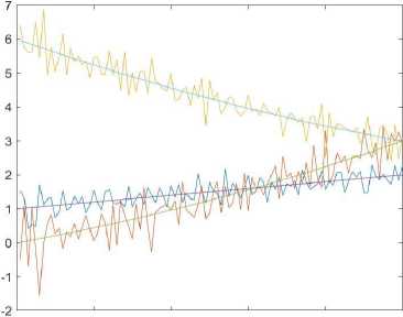
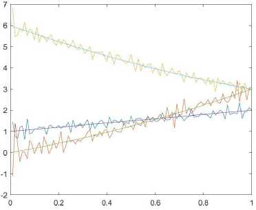
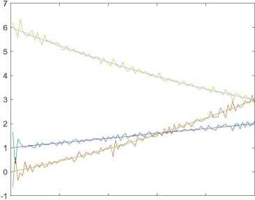
Based on the results of the experiments of the first group, it is difficult to estimate the dependence of the increase in the accuracy of calculations with an increase in the number of grid nodes. For the second group of data, we take data from the first group, add noise δ = 0 . 05, add additional measurement Ф 3 = x ² and the function а з = ( t — 2) 2 + 2. As for the previous group, we will present the results in the form of triplets, (Table 2).

Results for second group				Table 2
grid	ε α	ε u	T τ
Z 1	1 , 66	0 , 09	3 , 88
Z 2	1 , 34	0 , 05	9 , 45
Z 3	0 , 7	0 , 03	49 , 3
Z 4	0 , 39	0 , 01	1061 , 2

The results shown in Fig. 1. For brevity, we only display graphics and tables with the results of calculations α i .

О             0.2            0.4            О.В            0.8             1

b)

a)

О           0.2          0.4           0.6          0.8           1

c)

d)

Fig. 1 . The results for second group of data: a) Z 1 ; b) Z 2 ; c) Z 3 ; d) Z 4

As we can see 5-percent random noise increases the calculation error quite significantly, but despite this, the calculation results repeat the trends of the desired functions. It is now clear that increasing the number of nodes has a positive effect on accuracy, but a negative effect on the computation time. Based on this, for further experiments we will use only grid Z 3 .

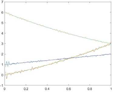
For the third group of data, we take coefficients of the equation: a = ( x + 1)( y + 1) / (1 + t ), b l = ^(t + ^{1)( x} + ^{1) 2} , b 2 = ^(t + ^{1)( y} + ^{1) 2} , c ll = ^{( x} + ^{1) / ( t} + 1), c 22 = ^(y + ^{1) / ( t +} 1), f = ^{0 ;} the desired functions a i = — t + 2, a 2 = 3( t — 0 , 6) 2 + 1, а з = 3( t — 0 , 5) 3 + 1 , 5; additional measurements and random noise are the same as in the second group.

The graphs are shown in Fig. 2 and the result is the triplet: (0 , 66; 0 , 05; 42 , 9).

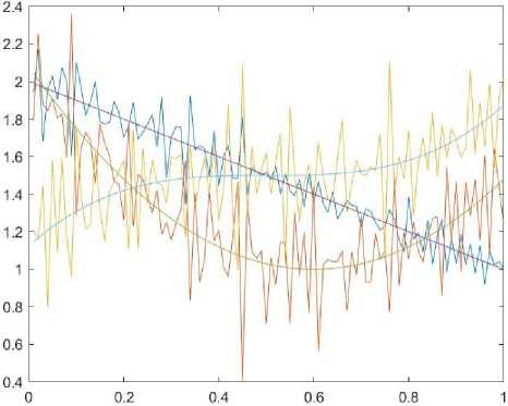
Fig. 2 . The results for third group of data

Conclusion

Using theoretical results on well-posedness of the problem, we construct a numerical algorithm for recovering the flux on the boundary with the use of integral observations of the concentration. It is based on the conventional methods (in our case FEM and difference schemes). The results of numerical experiments are presented. The obtained results reveal the accuracy, efficiency, and robustness of the proposed algorithm. It is stable under random perturbations of the data.