Investigation of the Wave Nature of the Ukrainian Stock Market

Published Online February 2012 in MECS

Under the conditions of heightening complexity, dynamism and stochasticity of the processes in the socioeconomic systems, a significant part of the economic science conceptions has to be reconsidered. This fact has been reflected in the revision of the classical paradigm of economics and the adoption of a neoclassical one. The difference between these two paradigms is in the understanding of the essence of economical processes. The classical approach to the dynamics of changes has been based on the property of determinacy of the open systems, i.e. the behavior of those was uniquely determined by the cause-and-effect interrelation. It means that the future of such a system is rigidly and uniquely determined by the past: Under the condition of knowing the principles the system development, the future behavior of the system can be forecasted unambiguously. Each unpredictable event was considered as an accessory factor and the chaotic behavior was treated in a destructive manner. The neoclassical paradigm is based on the nonlinear approach to the study of open systems, which comprises the powerful mechanisms of positive and negative feedbacks; the later can then self-organize and further develop. The nonlinear behavior of the socio- economic systems in the space and time means the multivariance of the development directions and also causes irreversibility of the evolutional processes.

Within the framework of this new paradigm of scientific investigations, the methodology and tools of the economical sciences were significantly changed. These factors have served as a basis for the wide usage of the tools peculiar to the catastrophe theory, wave theory, cycle theory, evolution theory, chaos theory and for the construction of new economic theory branch – the economical dynamics. The most noticeable investigations in this area was carried out Refs. [1-7].

The methodology is mostly expedient for the investigation of the stock market processes. This is because these markets, being the constituents of the financial ones, are highly stochastic. Displaying the current tendencies in the country development, these markets are governed by the general principles of the cyclic development and acquire the wave-like cyclic character. It is worth noticing that the waves are ordered and determinate oscillations, but the cycle is the particular case of the wave and this cycle is characterized by the constant period and amplitude.

The stock market is the structural element of the national economy, which involves the conflict of interest of different subjects, in particular - of investors. The investors compose the scenario of the market behaviour by using various mathematical tools which allows one to forecast the tendency changes of the share market. At present, short-tem adaptive forecasting models, fractal and spectral methods and models of fast processes (stock chaos) have gained the highest popularity.

The aim of the current article to investigate the nature of nonlinear cycles corresponding to changes which take place in the Ukrainian stock market. These changes arise due to the synergetic effect of the stochastic influence of internal and external factors.

The following tasks are addressed in this study:

• (i)    The wave nature of Ukrainian stock market;

• (ii)    The fractal analysis of PFTS index time series;

• (iii)    The determination and analysis of the cyclic components in the prices series of Ukrainian liquidly enterprise shares;

• (iv)    The determination of the stock market stability in the short-term period.

• II.    Methodology

The correlation between the tasks and mathematical tools are shown in Table I.

TABLE I.        Mathematical tools for the

INVESTIGATION

Tasks	Mathematical tools
investigation of the wave nature of Ukrainian stock market	The algorithmic model
analysis of the fractals in the PFTS index time series	R/S analysis
determination and analysis of the cyclic components in the prices series of the liquidly enterprises shares of Ukraine	ADF test Spectral analysis Time series analysis
determination of the long-term and shortterm cycles	Analysis of the coefficient
Determination of the stability of the stock market in the short-term period	Analysis of the coefficient

We use an algorithmic model for the investigation of the nonlinear nature of stock market. First, this model is considered as the combination of all research tasks, but from the other side the other it is a separate problem for the investigation. Figure 1 presents the unification of the stages for the algorithmic model.

Each stage of the model has a complex character since it includes the complex of algorithms and models for the research of the stage local purpose.

The purpose of the investor is the formation of the adaptive behavior which includes long-term and shortterm interests. Determination of the long-term and shortterm cycles in the dynamics of shares supports the balance between the interests of the investor.

Stage 1. Formation of the factor space for the investigation I PFTR , { P td }

I PFTR , { P td }

PFTR

It

Stage 2. Analysis of supporting tendency in the time series of the PFTS index

Stage 3. I nvestigation of the time series wave nature for shares and PFTS index

R/S analysis

Spectral analysis of the time series

Interpretation of the results

T

Stage 4. Determination of the long-term and short-term harmonics in the time series

I P^FTR , { P td }

Stage 5. Determination of the stability of the Ukrainian stock market

Figure 1. Algorithmic model of the investigation

Below we analyze the stages of the algorithmic model.

Stage 1. Formation of the factor space of investigation .

The purpose of the first stage is the formation of the investigation factor space. The indexes are the main indicators of the business activity of stock market. The PFTS index is the index of the secondary stock market. It shows the permanent change of shares capitalization. The shares of the most liquidly Ukrainian enterprises compose the structure of PFTS index. This structure has slightly changed for the last five years.

The analysis of the industry branches shows that energy, metal working, oil and gas, machine building enterprises are the leaders of the trade in PFTS market [12]. Besides, the Ukrainian market has been gradually integrating to the global stock market and the PFTS index has been included in the IFC Frontier index. Therefore the choice of PFTS index is expedient for the investigation of the nonlinear wave nature processes for the Ukrainian stock market.

The analysis of the stock market general tendency is quite important for the formation of investor behavior but at the same time it is necessary to carry out the analysis of other accompanying factors. In addition, the activity of the trade and shares value have to be analyzed. Such an approach allows one to determine both the attractive period for the activity of the investors and the attractive shares for formation of portfolio.

The structural analysis of the PFTS index in the 2005th year demonstrates the ten biggest enterprises of Ukrainian market, which are the “blue chips”.

TABLE II.        The structure of the PFTS index (2005)

Enterprises	Ticker	K	Price, UAH	+/-	Weight in PFTS index, %
Ukrtelekom	UTEL	0.071	1.045	2.02%	19.31
Nignydniprovskiy tube rolling plant	NITR	0.386	62.651	0.32%	18.05
Ukrnafta	UNAF	0.080	299.48	0.16%	17.96
Zaporigstal	ZPST	0.195	6.032	-0.27%	13.75
Concern Stirol	STIR	0.178	123.25	-0.40%	8.26
ZahidEnergo	ZAEN	0.299	150.45	3.76%	7.96
DniproEnergo	DNEN	0.239	378.450	+2.28%	4.92
KiyvEnergo	KIEN	0.372	7.678	-4.02%	4.29
CenterEnergo	CEEN	0.217	3.741	1.19%	4.15
DonbassEnergo	DOEN	0.142	29.000	3.20%	1.35

Note: K – the weight of the shares in the government property.

The course value of these shares is to be analyzed since these shares are most liquid and attractive for the investors.

Therefore the factor space of the investigation is the following cortege:

Pr = (i P™ , { p ,^d }                       (1)

where        IPtFTR - the time series of the PFTS index;

{ p _t ^d } - the set of the time series of the course value of the shares for the “d” enterprises.

Stage 2. The analysis of supporting tendency in the time series of the PFTS index.

We analyze the fractals in the time series of the PFTS index at the second stage. We utilize the method of normalized scope (R/S method) for our investigation. The so-called Hurst coefficient (H) is the base of the R/S method [7]. The interval of alternation for the Hurst coefficient is [0, 1]. Therefore this coefficient is the criteria of the classification of time series which can be either white noise, or persistent or non-persistent time series.

Table III shows the characteristics (the Hurst coefficient and the correlation coefficient) for the different kinds of time series.

TABLE III.       Criteria for the determination of the

PROCESS

Criteria		Name of the process	Verbal aspects of the process
Н	С(t)
Н = 1/2	С(t) = 0	White noise (Brownian process)	Last and future differences of the time series are independent and miscorrelated. The trend is not contained in the time series. This process is Gaussian process with independent variables, white noise.
Н < 1/2	C(t) * 0	Non-persistent process	This process is the stochastic process. If the time series increases, then time series will decrease in the future. The time series is characterized by the high level of the tendency change. If H ^ 0.5 then this time series is the white noise.
Н > 1/2	C(t) * 0	Persistent process	The last tendency is the permanent tendency in the future. Hence the persistent stochastic processes show the stability tendency with the low level noise. Persistent processes characterize the periodicity of the tendency.

Stage 3. Investigation of the wave nature of time series for the shares and PFTS index .

At the third stage we single out the cyclic components from the time series. The first step of the investigation of cyclic components consists in the analysis of the stationarity of time series. The mean value, deviation and covariance are the indicators of stationarity or non stationarity of the time series. The series is stationary if the mean and autocovariance of the series do not depend on time.

The conditions of the stationarity are: Ey t = ц , var(y t ) = у o , cov⁽y t ,y t - 1 ) = Y j

The special tests for analysis of the stationarity are: Dickey-Fuller test (DF), Augmented Dickey-Fuller test (ADF) and Phillip-Peron test (PP). In this investigation we used the Augmented Dickey-Fuller test. The test is carried out by the estimation of equation with y t _{- 1} subtracted from both sides of this equation:

A y t = ц + yy_t - 1 + e t           ⁽²⁾

where         μ, γ are the parameters of the model

• ( y = 1 - p ); e_t is assumed to be a white noise.

The null and alternative hypotheses are:

H o : у = 0

H 1 : у <  0

While it might appear that the test can be carried out by performing a t-test on the estimated γ , the t -statistic under the null hypothesis of a unit root does not have the conventional distribution. Dickey and Fuller (1979) showed that the distribution under the null hypothesis is nonstandard, and simulated the critical values for selected sample size. More recently, MacKinnon (1991) implemented a much larger set of simulations than those tabulated by Dickey and Fuller. The null hypothesis of a unit root is rejected against the one-sided alternative if the t -statistic less than a critical value.

After checking the stationarity of the initial time series by using the spectral analysis –the Fourier decomposition – we compose the cyclic component models. The algorithm for the search of these models is given in figure 2.

Step 1. Time series stationarity check I PFTR , { P td

Step 3. Construction of the harmonics spectrum and cyclic component models

Ceclt C ec l

M _PFTS , {M _d }    1..10

Figure 2. Algorithm for the composition of the cyclic component models.

In this case the cyclic component is the composition of different cycles, which can be presented as:

fl, ^           f ^

C(t)=E akcos — (t - i)| + £ bksin — (t -1)1 (4) k     I Tk     J k     I Tk     J where T is the period a separate cycle harmonic.

The quantity of harmonics is to be determined via the statistical significance of each harmonic. This allows us to form the Fourier series by employing the significant harmonics only.

The forth and fifth stages of the model are supposed to distinguish the most significant cyclic harmonics of the corresponding time series and to determine the stability of the Ukrainian stock market based on the weight of the long-term and short-term harmonics. This analysis allows the investor to make up or modify the share portfolio that is adequate to the market tendencies, and therefore to substantiate the market behavior. As the market stability criterion, one can use the ratio of the long-term and shortterm harmonics weights in the cyclic decomposition of the PFTS index, i.e.

long - term harmonic weight 1 short - termharmonicweight ^.

This is because the domination of the long-term harmonic in the cyclic component of the series investigated does not affect essentially on the change of the major tendency in the short term period. In this paper we understand the conservation of the dominant tendency in the short term period as the stability of the market development.

For the market stability analysis we utilize the following classification:

• i.    long-term harmonic with the period from 4 to 12 months;

• ii.    short-term harmonics with the period from 1 to 3 months.

The domination of either first or second type of harmonics allows one to determine the most attractive kind of the investor portfolio, which can be either of the conservative-aggressive or aggressive-conservative type correspondingly. Separation of the long-term and shortterm harmonics in the time series of the shares permits to compose the recommendations for the investor on how to gain the balanced structure of the shares portfolio oriented towards the support of either liquidity or profitability.

III.    Results

• A.    The investigation of the PFTS index time series for the determination of the supporting tendency.

The calculations of the Hurst coefficient for the daily PFTS index time series (for the period from 13.10.1997 to 13.09.2005, 1843 cases) showed that the series investigated is persistent, i.e. it contains the fractals. These conclusions are confirmed by the regression line tilt (Fig.3) and the Hurst coefficient values: H = 0,9935

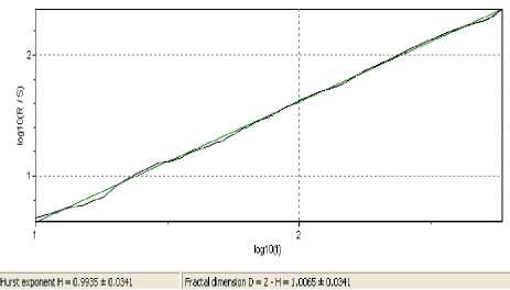
Figure 3. Regression line, Hurst coefficient for the initial series

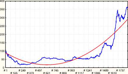
Figure 4. The time series of the PFTS index and the second-order polynomial approximation

B.    Investigation of the wave nature of the time series.

Step 1. The series stationary check. To determine the presence and to single out the cyclic components in the time series of the enterprises analyzed (Table 2) we perform the stationary check by means of the ADF test (Table IV).

TABLE IV. ADF test statistics

Ticker (yt)	L a g	Test equation
		y t = py t - 1 + Et		y t = a + py t - 1 + Et		y t = a + Ф t + py t - 1 + E t
		y t	A yt	y t	A y t	yt	A y t
CEEN	3	-1.04	-7.38**	-2.25	-7.42**	-0.21	-7.94**
	4	-1.08	-7.30**	-2.29	-7.29**	-0.39	-7.77**
DNEN	3	0.74	-5.07**	0.15	-5.10**	0.69	-5.92**
	4	0.80	-4.60**	0.05	-4.65**	0.62	-5.23**
DOEN	3	1.02	-8.36**	0.09	-8.40**	-0.36	-9.05**
	4	0.88	-5.84**	-0.04	-5.88**	-0.05	-6.51**
KIEN	3	0.05	-9.74**	-2.11	-9.72**	-2.71	-9.88**
	4	0.04	-7.96**	-1.84	-7.94**	-2.49	-8.11**
NITR	3	3.37**	-4.78**	0.51	-5.50**	-1.22	-5.60**
	4	2.63**	-4.11**	0.50	-4.64**	-1.81	-4.76**
STIR	3	1.17	-9.33**	-1.16	-9.47**	-2.26	-9.45**
	4	1.26	-8.13**	-0.92	-8.31**	-2.00	-8.29**
UNAF	3	2.72**	-7.43**	1.13	-7.91**	0.30	-8.00**
	4	2.69**	-5.71**	1.25	-6.13**	0.54	-6.28**
UTEL	3	0.69	-7.86**	-0.21	-7.92**	-1.15	-8.09**
	4	0.80	-6.99**	-0.12	-7.03**	-1.05	-7.22**
ZAEN	3	1.15	-8.14**	0.19	-9.22**	-1.20	-9.61**
	4	1.24	-8.14**	0.31	-8.25**	-1.10	-8.72**
ZPST	3	-0.28	-6.41**	-2.27	-6.40**	-2.78	-6.62**
	4	-0.25	-6.88**	-2.52	-6.86**	-3.05	-7.02**
PFTS	3	3.45**	-5.23**	2.43	-5.93**	0.54	6.29**
	4	2.88**	-4.33**	1.82	-4.91***	0.34	-5.22**

Note: ** – ADF test statistic more than 1% Critical Value;

Visual analysis of the time series (Fig.4) allowed as to put forward the hypothesis of the presence of the nonlinear trend. This hypothesis was confirmed by the approximation of the initial time series by the second-order polynomial function.

As a criterion of the validity of the model composed we used the multiply correlation coefficient with the value R = 0,9. Hence the trend model of the PFTS index has the following form: Y= 88,48 – 0.2252 t + 0,0002 t2

Analysis of time series I™ , { P^d } shows that all time series are non-stationary because ADF test statistic is less than 1% Critical Value. Thus this time series contains the trend. This inference also confirmed the computations of the ADF test for the 1^st differences, and this proves the fact that the series become stationary after singling out the trend

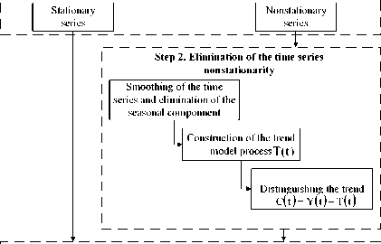
Step 2. Elimination of the non-stationary series.

For the purpose to eliminating the trends from the series let us decompose the series into the four components: the trend one (T(t)), the cycle one (C(t)), the seasonal one (S(t)) and the irregular one (I).

As the decomposition model we apply the additive one insofar as the series oscillation amplitude over the long-term period is stable. The model itself has the form:

Y ( t ) = T ( t ) + C ( t ) + S ( t ) + 1 (6)

For the sake of refinement of the initial series of the season component one can perform the smoothing over the period n=5, which corresponds to the 5 work-days at the PFTS market.

Distinguishing the trend from the fitted series includes the selection of the type of the trend and estimation of its parameters. The criterion for the choice of the general trend model defines the multiply correlation coefficient. The Table V shows the selected trend equations and trend parameters. The estimations of the model parameters are shown in Table A.I from Appendix.

TABLE V.       Trend models

Ticker	Equations	Correlation coefficient
CEEN	CEEN ( t ) = 1.042 — 0.0042t + 0.0000112t 2	0.957
DNEN	DNEN ( t ) = 66.382 — 0.28357t + 0.00104t 2	0.865
DOEN	DOEN ( t ) = 4.97969 — 0.0079t + 0.00000014t3	0.851
KIEN	KIEN ( t ) = 1.489329 — 0.012024t + 0.000185t2 — — ( 1.08E — 06 ) t3 + ( 2.14E — 09 ) t4	0.845
NITR	NITR ( t ) = 4.61464 + 0.026161t	0.961
STIR	STIR ( t ) = 11.10567 + 0.07786t — 0.000137t 2	0.852
UNAF	UNAF ( t ) = 33.142 — 0.032653t + 0.000462t2	0.915
UTEL	UTEL ( t ) = 0.151352 + + ( — 3.14E — 06 ) t2 + c ( 1.59E — 08 ) t3	0.831
ZAEN	ZAEN ( t ) = c21.83541 — 0.110770t + 0.000512t2	0.866
ZPST	ZPST ( t ) = 1.332383 — 0.0233399t + 0.000540t2 — — ( 5.05E — 06 ) t3 + ( 2.03E — 085 ) t4 — ( 2.92E — 11 ) t5	0.866
PFTS	PFTS ( t ) = 306.3156 + 0.001818t2	0.894

The analysis of the model parameters (Table A.I) and the adequateness of the model (Table V) show that all the model parameters are statistically significant ones, and the multiply correlation coefficients are within the norm limits. All these facts demonstrate the adequateness of the trend model.

The actual, fitted and residual dates of the PFTS index are shown in Fig. 5. The residuals of the series contain the cyclic component.

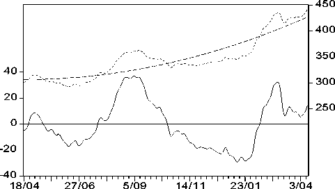
Residual Actual Fitted

Figure 5. Actual, fitted and residual dates of the PFTS index

The condition for the usage of the Fourier analysis for the cyclic component decomposition is the stationarity of the series. Then we carry out the second ADF-test for residuals of the series (Table A.II).

The results of the ADF test read:

• (i)    all series are the stationary ones with the 1% critical value for none and intercept test equations;

• (ii)    all series are the stationary ones with the 5% critical value for trend and intercept test equations.

Hence one can apply the Fourier analysis for the series residuals to study the harmonics of the cyclic component.

Step 3. Construction of the harmonics spectrum and cyclic component models.

The estimation sine and cosine coefficients together with the spectral densities are given in Table A.III. Below we present the model of the cyclic components for the PFTS index time series.

PFTS_C ( t ) = — 0.7967cos

2n t 258

+

2 n + 9.0659sin ---1,

258 1

+ 9.8624cos 2n _129t] — 18.826sin 2n , _129 1 _ + 3.315cos 2n, _ 86 11 _ + 2n Г2 n 2n + 0.1281sin t — 7.59cos — t— 0.1274sin t — 86 1 J _ 64.5 1J _ 64.5 1J .            Г 2n 2П 2 71 — 1.604cos t + 2.3825sin t + 0.354co s — tl + 51.6 1J .51.6 1 _43 1 Г 2П 2n Г 2n 1 + 4.227 sin —t, + 1.399cos — ----1, + 0.029sin t 43 1J _ 36.86 1J _ 36.86 1 where        t1 = t — 1

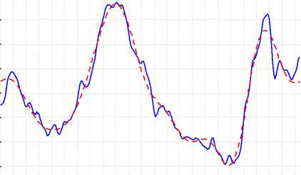
The model includes seven most significant harmonics for the cyclic component of the PFTS index. As the criteria for the selection of harmonics we take the values of the spectral density and the correlation coefficient. We would like to emphasize that the first five harmonics are the same for all series (see Table A.III, A.IV). This means that the coevolutional effects are present in the dynamics of the Ukrainian stock market. The plot for the residuals and the cyclic component estimated PFTS index time series is shown in Fig. 6. The plot for the shares time series is shown in Figs. A.1-5, see Appendix.

Line Plot (Findecon2006_Trend 35v*258c)

-10

-20

-30

-40

4/18/05      6/7/05      7/27/05      9/15/05      11/4/05      12/26/0      2/14/06      4/5/06

Fi

gure 6. Residuals and cyclic component for the PFTS index time series

• C.    Separation of the short-term and long-term cycles in the time series and determination of the stock market stability.

The Fourier decomposition allows one to separate the most significant harmonics in the share time series. The harmonic characteristics can be written by the following cortege:

Cycle s =< tSXT >  (7)

where Сycle _i ^s is the i -th harmonics of the action with label s ; t_i ^s is the initial value of the cycle; A_i ^s is the cycle amplitude and _{T i} ^s is the cycle periodicity.

In the current study the significance criterion for the harmonic is the cycle amplitude. Using this one then can distinguish the shares which correspond to the short-term and long-term investor purposes.

The values of the amplitude obtained for the most significant harmonics of the time series are given in Table VI.

TABLE VI.       Estimation of the amplitude and

SIGNIFICANT OF HARMONICS

T	258	129	86   64,5 51,6			43 6,86 25,8 23,45 21,5
CEEN
A	0,02	0,02	0,02	0,02	0,01	0,01	0,01
S	19,1	18,7	19,8	17,5	7,09	9,45	8,14
DNEN
A	1,13	2,58	1,05	0,66	0,70	1,32	1,11
S	13,2	30,1	12,3	7,73	8,23	15,3	13,0
DOEN
A	0,05	0,15	0,09	0,04	0,10	0,02		0,04
S	9,71	30,0	18,3	8,90	19,7	5,22		8,06
KIEN
A	0,01	0,04	0,02	0,04	0,02	0,04	0,01
S	1,30	21,1	10,3	25,2	10,2	24,5	7,19
NITR
A	0,54	0,36	0,05	0,37	0,06	0,07	0,09
S	34,4	23,0	3,35	23,9	4,29	4,65	6,24
STIR
A	0,79	2,13	0,99	0,32	0,40				0,43	0,44
S	14,4	38,6	17,9	5,82	7,30				7,81	7,98
UNAF
A	2,16	2,90	1,13	1,04	0,46	0,96	0,01
S	24,9	33,4	13,0	12,0	5,31	11,0	0,16
UTEL
A	0,00	0,01	0,01	0,01	0,01	0,01	0,01
S	4,01	30,7	8,47	15,3	19,4	14,7	7,22
ZAEN
A	0,59	1,23	0,73	0,91	0,57	0,79	0,26
S	11,6	24,2	14,3	17,8	11,2	15,5	5,11
ZPST
A	0,00	0,02	0,03	0,04	0,02	0,01			0,02
S	0,55	12,24	23,1	24,4	15,0	9,63			14,8
PFTS
A	9,10	1,25	3,31	7,592	2,87	4,24	1,39
S	18,28	42,69	6,66	15,25	5,77	8,52	2,81

To determine the stock market stability and single out the shares which possess the most significant long- and short-term cycles, we estimated the weight of the long-and short-term harmonics in the cyclic components of the series investigated (Table VII).

Inasmuch as the weight of the long-term harmonics in the cyclic component of the PFTS index time series occupy 68%, we can make the inference concerning the stability of Ukrainian stock market in a short-time period.

TABLE VII.      Weights of the harmonics in the cycles

Ticker	Weight of the long-term harmonic	Weight of the shortterm harmonic
CEEN	57,716	42,285
DNEN	55,635	44,365
DOEN	58,088	41,911
NITR	60,887	39,113
STIR	71,064	28,936
UNAF	71,422	28,577
UTEL	43,224	56,776
ZAEN	50,252	49,748
ZPST	35,993	64,007
KIEN	32,789	67,21
PFTS	67,646	32,353

Under such conditions it is pertinent to form the conservative-aggressive portfolio having the following structure:

• (i)    the conservative part is aimed to maintain the portfolio liquidity as a whole and involves the shares of the following enterprises: CEEN, DNEN, DOEN, NITR, STIR, UNAF ;

• (ii)    the aggressive part is aimed to maintain the profitability and includes the shares of the following enterprises: UTEL, ZPST, KIEN .

IV Conclusions .

To sum up, the from the analysis performed the following findings can be outlined:

• (1)    On the basis of the Hurst coefficient estimation we have deduced that the daily time series of the PFTS index over the period 03.10.1997 – 13.09.2005 is the persistent one, which means that it includes the fractality (the ability to maintain the stable tendency of development). Aside from this, the current tendency has a nonlinear character which supports the wave nature of the Ukrainian stock market development.

• (2)    The algorithmic model for the investigation of the wave nature of the stock market is a tool for the formation of the adequate investor behavior. It allows one to determine the structure of the shares portfolio, which combines the liquidity and profitability criteria.

• (3)    The separation of the most significant harmonics in the PFTS index and share series allowed one to determine the most expedient kind and structure of the portfolio.

To our belief, the future investigations of the wave nature of stock market consist in the development of methodological approaches for the investor strategy. These investigations should involve the forecasting of the crisis points of stock market based on the account of stochastic macroeconomical influence and tendencies in the development of the foreign stock markets.

Appendix