Landmarks in Hybrid Planning

Published Online November 2013 in MECS

The field of Artificial Intelligence (AI) planning provides a large variety of methods to construct plans of actions and reason about plan elements and plans [1]. There are two popular paradigms: classical state-based planning [2] and Hierarchical task network (HTN) [3].

The objective of classical state-based planning is to achieve a given set of goals. These goals are represented as a set of positive and negative literals in the propositional calculus. Also, the initial state is expressed as a set of literals. In classical state-based planning, actions are expressed using what are known as STRIPS operators [2]. Each action consists of two parts. The first part is precondition that must be true before the action can be executed. The second part is a set of effects that change the state of the world. Both the preconditions and effects can be positive or negative literals.

An HTN planning [3, 4] features another important principle of intelligent planning, namely abstraction. HTN planning is based on the concepts tasks and methods "i.e. predefined standard solutions for these tasks". Here, plan generation is a top-down refinement process that stepwise replaces abstract tasks by appropriate (abstract) solution plans until an executable action sequence is obtained. HTN planning is particularly useful for solving real-world planning problems since it provides the means to immediately reflect and employ the abstraction hierarchies that are inherent in many domains.

In classical state-based planning, the publications of the graph plan algorithm [5] and the International Planning Competition(IPC) [6] provided a strong development towards heuristic forward-search-based planning [7, 8, 9, 10]. They exploit knowledge that gained by pre-processing a planning domain and/or problem description to reduce planning effort.

The most popular pre-processing concept in classical state-based planning is the landmark. Landmarks are facts that must be true in every solution of a planning problem. The landmark concept was inspired by Porteous et al. [10] and further developed to extract landmarks and orderings between them from a planning graph of the relaxed planning problem [11, 12]. Other strands of research arranged landmarks into groups of intermediate goals to be achieved [13] and extended the landmark concept to so-called disjunctive landmarks[14, 15]. A disjunctive landmark is a set of literals any of which has to be satisfied in the course of a valid plan. A generalization of landmarks resulted in the notion of so-called action landmarks: actions that occur in every solution of a planning problem [16, 17]. Recently, the landmark information is used to compute heuristic functions for a forward searching planner [16, 18] and investigate their relations to critical-path-, relaxation, and abstraction-heuristics [19, 20, 21, 22]. In summary, it turned out that the use of landmark information can significantly improve the performance of classical state-based planners.

Recently, pre-processing technique is used to perform some pruning of the search space before the actual search is performed. Recently, There is only one technique has been introduced which restrict the domain and problem description of an HTN problem to a smaller subset, since some parts of the domain description might be irrelevant for the given problem at hand[23].

In hierarchical planning, landmarks are mandatory tasks either abstract or primitive. For an initial task network that states a current planning problem, a pre-processing procedure computes the corresponding landmarks. It does so by systematically inspecting the methods that are eligible to decompose the relevant abstract tasks.

In this paper, a novel technique to integrate the concepts of classical and hierarchical landmark [10, 23] is presented. We will use this integration to exploit the concept of landmark in hybrid planning [24].

The hybrid planning paradigm is particularly well suited for solving real-world planning problems, as it fuses ideas from classical planning with those of HTN planning: many real-world problems are inherently hierarchical and can more easily and adequately be encoded in the HTN planning paradigm. However, parts of the domain might be non-hierarchical and could be modeled more adequately in the classical state-based paradigm. Hybrid planning fuses both, in that it allows for the specification of an initial task network and of compound tasks as in HTN planning, but also enables the arbitrary insertion of tasks to support open preconditions as in classical planning. In addition, hybrid planning extends HTN planning in the following way:

• •    Tasks may be inserted into any task network without the need of being introduced via decomposition. This allows to plan for partially hierarchical domain models and makes hybrid planning decidable as opposed to standard HTN planning [25]

• •    The compound tasks show pre- and post-conditions. Hence, they can be inserted into task networks thereby improving the search efficiency. The performance increase results from the fact that the decomposition method specify predefined standard solutions for the compound tasks post-conditions.

• •    A goal description can be specified like in the classical state-based planning.

Before introducing the concept of landmarks and their extraction in hybrid planning in Sec. 3, we will briefly review hybrid planning in general and our underlying framework in Sec. 2. In sec. 4, experiments on benchmark problems, which give evidence for a considerable performance increase gained through our technique are presented. The paper ends with some concluding remarks in Section 5.

• II.    The Hybrid Planning Framework

Our approach relies on a hybrid planning framework [24], which integrates the characteristic features of partial-order-causal-link (POCL) and htn techniques.

POCL planning is a technique used for solving classical state-based planning problems [26]. In POCL, plans are partially ordered sets of actions and show explicitly causal dependencies between actions. This allows for flexibility w.r.t. the order in which actions are finally executed and enables a human user to understand the causal structure of the plan.

An HTN planning allows for the specification of primitive tasks with preconditions and effects like in pure classical state-based planning, as well as abstract tasks which represent compound activities like manufacturing goods, and predefined standard solutions (decomposition methods) of these abstract tasks.

Our framework builds upon the syntax and semantics of the ADL language [27]. Accordingly, a task schema t(τ) = 〈prec(t(τ)), add(t(τ)), del(t(τ))〉 specifies the preconditions and effects of a task via conjunctions of positive and negative literals over the task parameters τ = τ1, ,τn,where applicability and state transformation of actions is defined as usual. In the hybrid setting, both primitive and abstract tasks show preconditions and effects, which enables the use of pocl planning operations even on abstract levels.

In our framework, a task network or partial plan P = 〈 S, <  , V, CL 〉 consists of a set of plan steps S, i.e., (partially) instantiated task schemata that carry a unique label to differentiate between multiple occurrences of the same schema - partially ordered by a set of ordering constraints <. V is a set of variable constraints that represent (in-) equations between variables or between variables and constants. Tasks(P) denotes the set of those task schema instances that are obtained from plan steps S by substituting all task parameters with constants for which a respective equation holds in V. CL is a set of causal links, as they are common in POCL planning: A causal link 〈 s i , ϕ ,s j 〉 indicates that ϕ is implied by the precondition of plan step s j as well as it is a consequence of the effects of plan step s i . p and is said to be supported this way. Methods m = 〈 t( τ ), P 〉 relate an abstract task t( τ ) to its implementing partial plan P. In general, multiple methods are provided for each abstract task. Please also note that no application conditions are associated with the methods, as opposed to other representatives of htn- style planning.

A hybrid planning problem has the structure Π = 〈 D, P_init, s_init, s_goal 〉 . It is formulated over a domain model D = 〈 T,M 〉 , i.e., sets of task schemata and decomposition methods, an initial and goal state description s init , s goal , and an initial partial plan P init . Plan generation then means to refine P init stepwise into a partial plan P = 〈 S, < , V, CL 〉 that satisfies the following solution criteria:

• 1.    P is a refinement of P init , i.e., it is a successor of the initial plan in the induced search space (see Def. 1 below) ,

• 2.    Each precondition of a plan step in S is supported by a causal link in CL,

• 3.    The ordering and variable constraints are consistent, i.e., <  does not induce cycles on S and the (in-) equations in V are free of contradiction,

• 4.    None of the causal links in CL is threatened, i.e., for each causal link 〈 s_i, ϕ ,s j 〉 the ordering constraints in <  ensure that no plan step s _k with an effect that implies ϕ can be consistently placed between plan steps s _i and s j , and

• 5.    All plan steps in S are primitive tasks.

An hybrid planning problem Π induces a space of plan refinements in which the planning system searches for a solution. Refinement steps include the decomposition of abstract tasks by their methods, the insertion of causal links to support open preconditions of plan steps as well as the insertion of ordering and variable constraints [28]. We call such a refinement step a plan modification.

Definition 1 (Induced Search Space). The directed graph PΠ = 〈 V Π, ℰΠ 〉 with vertices V Π and edges ℰΠ is called the induced search space of the planning problem Π iff (1) P init ∈ VΠ , (2) if there is a plan modification refining P ∈ VΠ into a plan P ' , then P ' ∈ VΠ and (P,P') ∈ ℰΠ , and (3) P Π is minimal such that (1) and (2) hold. For PΠ , we write P ∈ PΠ instead of P ∈ VΠ . In general, PΠ is neither acyclic nor finite.

Our refinement planning algorithm (Alg. 1) takes the initial plan of the planning problem Π as an input and refines it stepwise until a solution is found.

Algorithm 1: Refinement Planning Algorithm input : The sequence Fringe = (jR*h).

output: A solution or fail.

• 1    while Fringe = (Pi... P_n) / c do

• 2    Ft-/ⁿ”^tel(Pl)

• 3    if F = 0 then return Pi

(■t ..X) *- /м“Юп,( U /^“(t))

• 4                     teF

• 5    succ <— (арр1у(ж1. Pi)... apply(e'_n. Pi))

• 6    Fringe <- /^PunOnl(succ о (Pi... P„))

• 7    return fail

The fringe of the algorithm is a plan sequence 〈P1... Pn〉 ordered by the used search strategy. It contains all non-visited plans that are direct successors of visited non-solution plans. According to the used search strategy, a plan Pi leads more quickly to a solution than plans Pj for j > i. The current plan under consideration is always the first plan of the fringe. The planning algorithm loops as long as no solution is found and there are still plans to refine (line 1). Hence, the flaw detection function fFlawDet in line 2 calculates all flaws of the current plan. A flaw is a plan component that is involved in the violation of a solution criterion. In hybrid planning, the presence of an abstract task raises a flaw that includes that task, a causal threat consists of the causal link and the threatening plan step, and so on. If no flaws can be found, the plan is a solution and returned (line 3). In line 4, all plan modifications are calculated by the modification generating function fModGen, which addresses all published flaws. Afterwards, the modification ordering function fModOrd orders these modifications according to a given strategy. The fringe is finally updated in two steps: First, the plans resulting from applying the modifications are calculated (line 5) and are put in front of the fringe in line 6. Second, the plan ordering function fPlanOrd orders the updated fringe according to its strategy. This step can also be used in order to discard plans (i.e., to delete plans permanently from the fringe). This is useful for plans that contain unresolvable flaws like an inconsistent ordering of tasks. If the fringe becomes empty, no solution exists and fail is returned.

This approach defines its search strategy in an explicit manner as the combined result of the deployed modification and plan ordering functions. E.g., in order to perform a depth first search, the plan ordering strategy is the identity function (f^PlanOrd(p') = p' for any sequence P') , whereas the modification ordering strategy f^ModOrd decides, which branches to visit first. In this way, the plan ordering strategy is used to prioritize the plans; several strategies can be concatenated into cascades. The plan ordering strategy uses also its input sequence for tie-breaking: If two plans are invariant after application of the plan ordering function, the order given in the input is used. This set-up allows for constructing a rich variety of planning strategies.

• III.    Hybrid Landmark

As mentioned before in the text, classical landmarks are a set of facts, while hierarchical landmarks are a set of tasks either abstract or primitive. Obviously, we believe that integrating both techniques could result in an improvement of the planning process. In the following lines, we will show how to integrate them.

In our integration technique, we use the landmark technique which restricts the domain and problem description of an HTN to a smaller subset, since some parts of the domain description might be irrelevant for the given problem at hand [23].

For a given hierarchical planning problem Π = 〈 D, s init , P init 〉 , landmarks are the tasks either primitive or abstract that occur in every sequence of decomposition leading from the initial plan P _init to a solution plan.

Definition 2 (Solution Sequences). Let 〈VΠ, ℰΠ〉 be the induced search space of planning problem Π. Then, for any plan P ∈ VΠ, SolSeqΠ(P) := {〈P1... Pn〉|P1 = P, (Pi, Pi + 1) ∈ ℰΠ for all 1 ≤ i < n, and Pn ∈ Soln for n = l}.

Definition 3 (Landmark). A ground task t( τ ) is called a landmark of planning problem Π , if and only if for each 〈 P 1 ,...,P n 〉∈ SolSeq n (P init ) there is an 1 ≤ i ≤ n, such that t( τ ) ∈ Ground (S i ,V n ) for P i = 〈 S i ,< i ,V i ,CL i 〉 and P n = 〈 S n , < n ,V n ,CL n 〉 .

Landmark extraction algorithm (Alg. 2) starts by constructing a task decomposition graph (TDG) for a given planning problem Π . A TDG is a directed bipartite graph 〈 V T , V M , E 〉 with task vertices V T , method vertices V M , and edges E. A TDG should satisfies the following conditions:

• 1.    t( τ ) ∈ V T for all t( τ ) ∈ Ground(S,V), for P init = 〈 S,

• <, V, CL 〉 ,

• 2.    if t( τ ) ∈ V T and if there is a method 〈 t( τ ), 〈 S,<, V, CL 〉〉∈ M , then

• (a)    ( t( T ),{S,<,V* , CL» e V m such that V * 2 V binds all variables in S to a constant and

• (b)    (t( τ ), (t( τ ), 〈 S,<,V ',CL 〉〉 ) ∈ E,

• 3.    if 〈 t( τ ), 〈 S, <, V, CL 〉〉 ∈ V M , then

• (a)    t'( τ ') ∈ V T for all t'( τ ') ∈ Ground (S, V) and

• (b)    〈〈 t( τ ), (S,<,V,CL 〉〉 ,t'( τ ')) ∈ E, and

• 4.    〈 V T ,V M ,E 〉 is minimal such that (1), (2), and (3) hold.

It is worth mentioning the TDG of a planning problem Π is always finite as there are only many ground tasks. Note that, due to the uninformed instantiation of unbound variables in a decomposition step in criterion 2.(a), the tdg of a planning problem becomes in general intractably large. We hence prune parts of the tdg which can provably be ignored due to a relaxed reachability analysis of primitive tasks.

The extracted landmark tasks are organized in a table so-called landmark table. Its definition relies on a task decomposition graph, which is a relaxed representation of how the initial plan of a planning problem can be decomposed.

The landmark table is a data structure that represents a (possibly pruned) tdg.

Definition 4 (Landmark Table). Let 〈 V T ,V M , E 〉 be a (possibly pruned) TDG of the planning problem Π . The landmark table of Π is the set LT = { 〈 t( τ ),M(t( τ )),O(t( τ )) 〉 | t( τ ) ∈ V T abstract ground task }, where M (t( τ )) and O(t ( τ )) are defined as follows:

M(t( τ )) := {t'( τ ') ∈ V T | t'( τ ') ∈ Ground(S, V) for all 〈 t( τ ), 〈 S, < ,V,CL 〉〉 ∈ V M }

O(t( τ )) := {Ground(S, V) \ M(t( τ )) | 〈 t( τ ), 〈 S,< ,V,CL 〉〉∈ V M }

Each landmark table entry partitions the tasks introduced by decompositions into two sets: mandatory tasks M(t( τ )) are those ground tasks that are contained in all plans introduced by some method which decomposes t( τ ); hence, they are local landmarks of t( τ ). The optional task set O(t( τ )) contains for each method decomposing t( τ ) the set of ground tasks which are not in the mandatory set; it is hence a set of sets of tasks.

Note that the landmark table encodes a possibly pruned tdg and is thus not unique. In fact, various landmarks might only be detected after pruning. For instance, suppose an abstract task has three available methods, two of which have some tasks in their referenced plans in common. However, the plan referenced by the third method is disjunctive to the other two. Hence, the mandatory sets are empty. If the third method can be proven to be infeasible and is hence pruned from the tdg, the mandatory set will contain those tasks the plans referenced by the first two methods have in common.

The landmark extraction algorithm simply tests all primitive tasks for relaxed reachability, starting with the initial plan (the root of the TDG) and proceeding level by level of the TDG. If a task can be proven unreachable, the method introducing this task is pruned from the TDG and all its sub-nodes (and so forth). After all infeasible methods of an abstract task t have been pruned from the TDG, this task, its intersection, and the remaining tasks are stored into the landmark table.

Now, we will take a look, how this is achieved by our algorithm (Alg. 2): First, the landmark table and a set for backward propagation get initialized (line 1). Afterwards, each abstract task, which is not yet stored into the landmark table is considered level by level of the TDT (line 2 to 4). For the current abstract task at hand, line 6 to 8 calculate the intersection and the remaining tasks in the yet unpruned TDG according to "mondatory task set" and "remaining task sets". In line 8, we subtract the empty set from O(t), because we are only interested in the tasks, that are actually remaining; if there are no remaining tasks, O(t) should be empty, instead of containing an empty set. After the tasks introduced by decomposition of t have been partitioned into M (t) and O(t), these sets are analyzed for infeasibility. This test is performed by a relaxed reachability analysis. First, we study the primitive tasks of M(t) (line 9). If such a task can be proven to be infeasible, all methods of t become obsolete and can hence be pruned from the TDG (line 10 and 12). After this test, each remaining task set is tested for reachability. If an infeasible task can be found, only this specific method gets pruned from the TDG (line 13 to 17). If something was pruned, the loop (line 5 to 18) enters another cycle, because the set M(t) might have grown. If no more pruning is possible, the intersection and remaining task sets for t are stored into the landmark table in line 19. When storing an entry in line 20, it is checked whether the stored abstract task is feasible or not (an abstract task is infeasible if it does not have any methods left, i.e., if M(t) and O(t) are empty). If some abstract task could actually be proven infeasible, it is stored for backward propagation, because again all methods containing this abstract task can be pruned from the TDG and from the landmark table. Finally, if all abstract tasks are checked, the backward propagation procedure is called with the current landmark table and TDG in line 22.

Procedure propagate 3 takes as input the already filled landmark table, the possibly pruned TDG and a set infeasible of abstract tasks which have been proved infeasible due to no remaining methods in the TDG. It works tail-recursively and returns the final landmark table as soon as no propagation is possible (line 1). To this end, it first takes and removes some arbitrary task t' from the set infeasible. Because this abstract task was proven infeasible, all methods containing it have to be removed from the TDG. As a consequence of this pruning, the intersection and remaining task sets have to be updated; additionally, further propagation can now be possible. To calculate the methods that can possibly be pruned, all parent tasks of t' are identified (line 3). Then, for all these parents (line 4), the respective methods are removed in line 5. Because methods were removed, the intersection and the remaining task sets could have changed again. Hence, they are recalculated in line 6 to 8. Next, the the old landmark table entry of the current parent t is removed and replaced by the new one (line 9). In line 10, it is tested again, whether the new landmark table entry corresponds to an infeasible abstract task. If so, it is put into the set infeasible for later testing. The procedure is then called with the modified parameters in line 1.

Without a formal proof, we want to mention that algorithm 2 (i.e., the initial landmark table calculation as well as the backward propagation) always terminates. For the first part of the algorithm, this is easy to see because both loop conditions (line 2 and 3) cannot be modified within the loops. For the second part, i.e., the propagate procedure, we have to show that the set infeasible becomes empty eventually. This is the case because each task gets inserted at most once and will be removed at some point.

On the other hand, in order to extract classical landmarks (set of facts) from the same domain model and hybrid planning problem Π, we should transform the respective hierarchical domain into a classical domain model and transforms the given hybrid planning problem Π into a relaxed classical planning problem Π'=〈D', φ, sinit, sgoal〉, where domain model D = 〈T, M〉 translated into D' = 〈T, φ〉. The next section explains how to transform a hybrid planning problem and a respective hierarchical domain model into a classical planning problem and classical domain model.

Algorithm 2: Landmark Extraction Algorithm Input : A task decomposition Graph TDG. Output: The filled landmark table LT.

I LT 4— 0, infeasible 4— 0

2 for г 4— 1 to TDG.maxDepth() do

foreach abstract task t in level i of TDG do if LT contains an entry for t then continue repeat

Let M be the methods of t in the TDG.

A/(f) 4- П tn meai

OWe-^mlXfO} foreach primitive task t* E M(t) do if V can be proven infeasible then remove all m E M from the TDG. including all sub-nodes.

break foreach remaining task set r E 0(0 do foreach primitive task I' € r do if V can be proven infeasible then remove the method m = (t, P), with Tasks^P) = M(0 Ur from the TDG. including all sub-nodes.

continue until no method was removed from TDG

LT4-LT U{(t,Af (0,0(0))

if M (t) = 0(0 = 0 then

I infeasible 4— infeasible U (t)

A. DOMAIN TRANSFORMATION

An HTN planning domain will be translated into a classical planning domain as follows:

• •    By building a TDG .

• •    By translating each occurrence of an abstract task as described in the following paragraph; and translating each occurrence of a primitive task as described in the paragraph after next.

Input : A landmark table LT. a task decomposition graph TDG. possibly pruned, and a set of abstract tasks infeasible, which have been proved infeasible.

Output: the updated landmark table LT. in which methods are pruned that contain infeasible abstract tasks.

• 1    if infeasible = 0 then return LT

• 2    infeasible 4- infeasible \ (t'}- where

parents 4-{t|(t,Af (0,0(0) 6 LT, t'eM(0u (J r)

• 3                                             reo(o

• 4    foreach t E parents do

• 5    Remove all methods from the TDG. that contain t’ in its plan. i.e., all m = (t, P) with t' E Tasks! P).

• 6    Let M be the methods of t in the TDG.

  - M(t\ 4- O m

• ⁷     '' m£M

Translating occurrences of abstract tasks. Each occurrence of an abstract task t( τ ') will be translated into a new STRIP-style operator t new ( τ ') as follows:

• •    The execution of an abstract task t( τ ') is completed if one of its decomposition methods is achieved. The later one is achieved if and only if all its sub-tasks (i.e., t 1 , t 2 , ... ,t k ) are performed. Therefore, we will construct a new task instead of a decomposition method to ensure the execution of the respective method. The name of this new task has the form TaskRef - new - MethodName. The preconditions of

this task are all the artificial literals t 1 -solved,t 2 -solved, ...., t k -solved of sub-tasks in the respective method. In case of these sub-tasks are ordered together such as t 1 <  t 2 and t 2 <  t 3 , then the precondition of a new task has only the effect and artificial literal of the last task in the order constraints (i.e., effect(t₃) and t₃-solved) because the completion of other sub-tasks is considered by the translation of the order constraints as we will see later in this section.

• •    A new task has only a single add effect TaskRef - achieved which indicates that the execution of task which created instead of method is completed. Note that in case of there is a number of decomposition methods can decompose the same abstract task, then a number of new tasks are created based on the number of decomposition methods. All of these tasks have the same effect (i.e.,TaskRef - achieved).

• •    So, the precondition of a t new ( τ ') is the artificial effect of the task TaskRef-new - MethodName and its effect is TaskName - solved.

Translating occurrences of primitive tasks. Each occurrence of a primitive task t( τ ') is transformed as follows:

• •    A new task t_new ( τ ') is created without any change in its preconditions.

• •    It’s effect will be extended by adding a new literal t new - solved to the original effect.

The ordering constraints between instances of sub-tasks is translated by adding additional preconditions. For example, the ordering constraints between sub-tasks (t₁< t₂) is expressed by adding the literal t_1-new-solved to the preconditions of sub-task t₂. If sub-task t 2 is abstract task, the literal t 1-new -solved will be added to every sub-task that is generated from the decomposition of t 2 .

In order to ensure the new tasks either primitive or abstract are used at most once in any solution, we add a literal t new - achieved to the task precondition.

A hybrid planning problem Π = 〈 D, P init , s init ,s goal 〉 is transformed into a new STRIPS-style planning problem Π '= 〈 D', φ , s' init ,s' goal 〉 as follows:

• •    A new domain model has the structure D^' = 〈 T^', φ 〉 , where all tasks T and methods M in the original domain model are translated into STRIPS-style operator T^' using our transformation technique.

• •    All tasks in the initial plan P_init is translated by adding a new task, the so-called t - solve to the domain model D^'. The preconditions of t - solve is the effect of all root tasks in a tdg and its effect is a new literal, namely t - solve - achieved . This means, the new task t - solve assures the complete execution of all tasks in the initial partial plan P init .

• •    The original goal state s_goal is extended by adding the literal t - solve - achieved (i.e., s'_goal = s_goal U t - solve - achieved).

• •    The new initial state s' init is represented by the original initial state s init , and it is extended by the negative facts for all tasks in the new domain model D^' and   t - solve-achieved i.e., s' init = {s init Ս { t new - achieved |t ∈ T' and t new - achieved ∉ s init } Ս { t- solve - achieved }} .

So, the integration between classical and hierarchical landmark techniques will proceed in three steps as follows:

• 1.    By applying landmark algorithm [11] on the new planning problem Π ' and translated domain model D', the landmark algorithm proceeds in three steps. First, the relaxed planning graph(RBG) (i.e., the planning task is relaxed by ignoring all delete effects.) is built. This will be done by applying chaining forward from the initial state s' init in the planning problem n' until all goal literals in s^'_goal are achieved. Because the delete effects are ignored, the RBG does not include any mutex relations [8]. Second, the set of classical landmarks is extracted by applying candidate generation procedure. Third, the extracted landmarks are evaluated by applying filtering procedure to remove landmarks which fail the test. we extended this filtering algorithm to remove also the artificial literals out of the extracted landmarks.

• 2.    It is not hard to extract the actions A that can possibly achieve these landmarks (i.e., A = {a|a e T', landmark l ∈ eff(a)}).

• 3.    On the other hand, landmark table includes the landmark tasks that are produced from the original planning problem and domain model.

We use the set of action which extracted from classical landmark "in step 2" to refine the landmark table. To this end, we compared the primitive tasks which exist in the optional sets in the landmark table and remove all optional sets which have primitive tasks does not exist in the action set A.

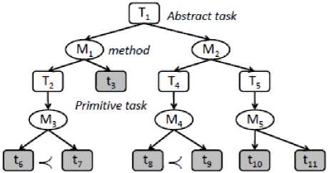
Fig. 1: Artificial Example

Example. In order to illustrate our transformation technique, let us consider a simple artificial example in Figure 1. Note that the abstract and primitive tasks are represented by capital and small letters respectively. The oval shape represents decomposition methods and < represents ordering constraints between sub-tasks. Assume that the abstract task T ₁ can be decomposed by two methods M 1 and M 2 . As depicted in table 1, these methods will be converted to new tasks so-called T 1 - new - M 1 and T 1 - new -M 2 . They have the same effect T 1 - achieved but with different preconditions. These preconditions confirm the execution of the sub-tasks in the respective decomposition method. Therefore, the precondition of the first new task T₁-new- M₁ is effect of primitive sub-task t₃ and the artificial effect T 2 - solved of abstract task T 2 . On the other hand, the decomposition method M 3 will be translated to task T 2 -new-M 3 with precondition eff (t 7 ) and its effect is T 2 - achieved. This is because task t 6 is ordered before t 7 then in our transformation technique the effect of task t 6 is added to the precondition of task t 7 . This means that the task t₇ cannot performed before task t₆ is completed firstly.

• IV.    Evaluation

In order to quantify the practical performance gained by our approach, we conducted a series of experiments with our planning framework. The experiments were run on a machine with a 3 GHz CPU and 256 MB Heap memory for the Java VM. Note that this machine has only one single processor unit.

Table 1: The result of transforming the artificial example from hierarchical to classical domain

Original tasks And methods	Translated Tasks
T 1	Name : T 1 - new Pre : T1 - achieved Eff: T 1 - solved
M 1	Name : T 1 - new - M 1 Pre : eff (t 3 - new) T 2 - solved Eff: T 1 - achieved
T 2	Name : T 2 - new Pre : T2 - achieved Eff: T 2 - solved

t 3	Name : t3 - new Pre: pre(t 3 ) Eff: eff (t 3 ) U t 3 - solved
M 3	Name : T 2 - new - M 3 Pre : eff (t7 - new) Eff: T 2 - achieved
t 6	Name : t 6 - new Pre: pre(t 6 ) Eff: eff(t 6 ) U t 6 - solved
t 7	Name : t 7 - new Pre : pre(t 7 ) U eff (t 6 - new) Eff: eff (t 7 ) U t 7 - solved
T 4	Name : T 4 - new Pre : T 4 - achieved Eff: T 4 - solved
T 5	Name : T 5 - new Pre : T 5 - achieved Eff: T 5 - solved
M 4	Name : T 4 - new - M 4 Pre : eff (t 9 - new) Eff: T 4 - achieved
t 8	Name : t 8 - new Pre: pre(t 8 ) Eff: eff(t 8 ) U t 8 - solved
t 9	Name : t9 - new Pre : pre(t 9 ) U eff (t 8 - new) Eff: eff(t 9 ) U t 9 - solved
M 5	Name : T 5 - new - M 5 Pre : eff (t10 - new) U eff (t11 - new) Eff: T 5 - achieved
t 10	Name : t 10 - new Pre: pre(t 10 ) Eff: ef f (t 10 ) U t 10 - solved
t 11	Name : t11 - new Pre: pre(t 11 ) Eff: ef f (t 11 ) U t 11 - solved

We evaluated the performance of our integration technique (HybridLM) along two dimensions: we compared the time needed to find a solution in comparison to conventional hierarchical planning (HP) and hierarchical landmark (HLM) [6]. The planning strategies we used are representatives from the rich portfolio provided by our planning environment [28]. We briefly review the ones on which we based our experiments.

Modification selection functions determine the shape of the fringe, because they decide about the (priority of the) newly added plan refinements. We thereby distinguish selection principles that are based on a priorization of certain flaw or modification classes and strategies that opportunistically choose from the presented set. The latter ones are called flexible strategies.

As for the flexible modification selections, we included the well-established Least Committing First (lef) paradigm, a generalization of POCL strategies that selects those modifications that address flaws for which the smallest number of alternative solutions has been proposed. From previous work on planning strategy development we deployed two HotSpot-based strategies: HotSpots denote those components in a plan that are referred to by multiple flaws, thereby quantifying to which extent solving one deficiency may interfere with the solution options for coupled components. The Direct Uniform HotSpot (du) strategy consequently avoids those modifications which address flaws that refer to HotSpot plan components. As a generalization of singular HotSpots to commonly affected areas of plan components, the HotZone (hz) modification selection takes into account connections between HotSpot and tries to avoid selecting modifications that deal with these clusters.

Plan selection functions control the traversal through the refinement space that is provided by the modification selection functions. The strategies in our experimental evaluation were based on the following five components: The least commitment principle on the plan selection level is represented in two different ways, namely the Fewer Modifications First (fmf) strategy, which prefers plans for which a smaller number of refinement options has been announced, and the Less Constrained Plan (Icp) strategy, which is based on the ratio of plan steps to the number of constraints on the plan.

Finally, For the strategies SHOP and UMCP, we used plan and modification selection functions that induce the search strategies of these planning systems: in the UMCP system [3], plans are primarily developed into completely primitive plans in which causal interactions are dealt with afterwards. The SHOP strategy [29] prefers task expansion for the abstract tasks in the order in which they are to be executed.

It is furthermore important to mention, that our strategy functions can be combined into selection cascades (denoted by the symbol +) in which succeeding components decide on those cases for which the result of the preceding ones is a tie. We have built five combinations from the components above, which can be regarded as representatives for completely different approaches to plan development. Please note that the resulting strategies are general domain-independent planning strategies, which are not tailored to the application of our integration in any way.

Table 2: Results for the UM-Translog domain

Problem	Mod. Sei	Plan Sei	HP	HLM	HybridLM
			Time	Time	Time
Pi	lef+hz	fmh+fmf	147	95	38
	Icf+ems	fmh+fmf	211	174	59
	lef+du	fhz+fmf	155	99	42
	hz+lcf	fhz+lcp+fmf	143	115	51
	SHOP Strategy		323	212	103
p2	lef+hz	fmh+fmf	182	140	65
	Icf+ems	fmh+fmf	269	216	112
	lef+du	fhz+fmf	216	129	63
	hz+lcf	fhz+lcp+fmf	299	162	79
	SHOP Strategy		595	257	136
№	lef+hz	fmh+fmf	301	236	122
	Icf+ems	fmh+fmf	443	298	158
	lef+du	fhz+fmf	314	251	197
	hz+lcf	fhz+lcp+fmf	469	413	293
	SHOP Strategy		558	433	307
№	lef+hz	fmh+fmf	377	203	98
	Icf+ems	fmh+fmf	613	206	142
	lef+du	fhz+fmf	483	370	187
	hz+lcf	fhz+lcp+fmf	458	507	293
	SHOP Strategy		479	416	242
PS	lef+hz	fmh+fmf	142	98	48
	Icf+ems	fmh+fmf	216	182	150
	lef+du	fhz+fmf	160	105	54
	hz+lcf	fhz+lcp+fmf	152	122	76
	SHOP Strategy		283	241	165
№	lef+hz	fmh+fmf	-	1237	654
	Icf+ems	fmh+fmf	-	1144	542
	lef+du	fhz+fmf	2755	1262	710
	hz+lcf	fhz+lcp+fmf	-	3544	1876
	SHOP Strategy		-	4005	2975
PT	lef+hz	fmh+fmf	149	92	54
	Icf+ems	fmh+fmf	225	179	86
	hz+lcf	fhz+lcp+fmf	153	120	74
	lef+du	fhz+fmf	173	104	58
	SHOP Strategy		911	177	112
№	lef+hz	fmh+fmf	1241	621	265
	Icf+ems	fmh+fmf	1805	513	276
	lef+du	fhz+fmf	1450	460	187
	hz+lcf	fhz+lcp+fmf	213	171	98
	SHOP Strategy		1911	874	208
PS	lef+hz	fmh+fmf	1240	215	128
	Icf+ems	fmh+fmf	1861	354	157
	lef+du	fhz+fmf	1074	159	143
	hz+lcf	fhz+lcp+fmf	198	172	79
	SHOP Strategy		1735	353	186
pio	lef+hz	fmh+fmf	1137	421	225
	Icf+ems	fmh+fmf	1425	677	398
	lef+du	fhz+fmf	1044	428	269
	hz+lcf	fhz+lcp+fmf	958	670	223
	SHOP Strategy		1282	863	532
pi!	lef+hz	fmh+fmf	507	435	134
	Icf-ems	fmh-fmf	413	471	257
	lef+du	fhz+fmf	749	621	128
	hz+lcf	fhz+lcp+fmf	777	609	298
	SHOP Strategy		821	450	169

Table 3: Results for the Satellite domain. The description x-y-z stands for a Satellite problem with x observations, y satellites, and z mode

Problem	Mod. Scl	Plan Scl	HP	HLM	Hybrid LM
				Time	Time
1-Ы	lef+hz	fmh+fmf	41	42	19
	lef+ems	fmh+fmf	51	53	25
	lef+du	fhz+fmf	72	72	33
	hz+lcf	fhz+lcp-fmf	62	60	36
	SHOP Strategy		67	61	34
2-1-1	lef+hz	fmh+fmf	788	708	289
	lef+ems	fmh+fmf	1631	1428	658
	lef+du	fhz+fmf	1319	1030	729
	hz+lcf	fhz+lcp+fmf	1699	1474	803
	SHOP Strategy		270	264	176
2-2-1	lef+hz	fmh+fmf	-	-	658
	lef+ems	fmh+fmf	-	-	925
	lef+du	fhz+fmf	-	3353	1548
	hz+lcf	fhz+lcp+fmf	-	-	784
	SHOP Strategy		-	1780	638
1-2-1	lef+hz	fmh+fmf	102	96	42
	lef+ems	fmh+fmf	291	290	147
	lef+du	fhz+fmf	98	90	43
	hz+lcf	fhz+lcp+fmf	178	138	72
	SHOP Strategy		254	230	126
2-1-2	lef+hz	fmh+fmf	3674	3651	1698
	lef+ems	fmh+fmf	-	-	872
	lef+du	fhz+fmf	2987	2971	1284
	hz+lcf	fhz+lcp+fmf	3278	2987	1429
	SHOP Strategy		-	3109	1702
2-2-2	lef+hz	fmh+fmf	875	659	298
	lef+ems	fmh+fmf	-	-	936
	lef+du	fhz+fmf	1978	864	398
	hz+lcf	fhz+lcp+fmf	422	357	152
	SHOP Strategy		-	-	731

• A. Benchmark Problem Set

We chose several planning domains for our experiments to ensure that the proposed approach is generally applicable. In particular, we used domains well known from the IPC plus domains from an ongoing research project. Satellite is a planning domain from the IPC for non-hierarchical planning. The hierarchical encoding of this domain regards the original primitive operators as implementations of abstract observation tasks. The Satellite domain model consists of 3 abstract and 5 primitive tasks, and includes 8 methods. Woodworking, also originally defined in the IPC's non-hierarchical manner, specifies in 13 primitive tasks, 6 abstract tasks, and 14 methods the processing of raw wood into smooth and varnished product parts. UM-Translog is a hierarchical planning domain that supports transportation and logistics. It shows 21 abstract and 48 primitive tasks as well as 51 methods. In addition to that, we also employed the so-called SmartPhone domain, a new hierarchical planning domain that is concerned with the operation of a smart phone by a human user, e.g., sending messages and creating contacts or appointments.

SmartPhone is a rather large domain with a deep decomposition hierarchy, containing 50 complex and 87 primitive tasks and 94 methods.

Table 4: WoodWorking domain: the problems define variations of parts to be processed

Problem	Mod. Sei	Plan Sei	HP	HLM	HybridLM
			Time	Time	Time
Pi	lef+hz	fmh+fmf	77	51	21
	lef+ems	fmh+fmf	90	76	32
	lef+du	fhz+fmf	108	92	41
	hz+lcf	fhz+lcp+fmf	201	179	156
	SHOP Strategy		98	76	31
№	lef+hz	fmh+fmf	-	2017	638
	lef+ems	fmh+fmf	591	324	123
	lef+du	fhz+fmf	1026	845	275
	hz+lcf	fhz+lcp+fmf	780	657	298
	SHOP Strategy		981	854	253
И	lef+hz	fmh+fmf	497	289	153
	lef+ems	fmh+fmf	871	765	352
	lef+du	fhz+fmf	-	-	478
	hz+lcf	fhz+lcp+fmf	985	789	256
	SHOP Strategy		-	-	549
P-i	lef+hz	fmh+fmf	3781	2892	1228
	lef+ems	fmh+fmf	2939	1876	548
	lef+du	fhz+fmf	1248	981	386
	hz+lcf	fhz+lcp+fmf		-	854
	SHOP Strategy		-	-	926
PS	lef+hz	fmh+fmf	-	-	2076
	lef+ems	fmh+fmf	-	-	1382
	lef+du	fhz+fmf	3761	3569	1693
	hz+lcf	fhz+lcp+fmf		-	658
	SHOP Strategy		-	-	497
PB	lef+hz	fmh+fmf	-	3215	925
	lef+ems	fmh+fmf	-	-	-
	lef+du	fhz+fmf	-	-	1954
	hz+lcf	fhz+lcp+fmf	2617	1513	429
	SHOP Strategy		-	2915	631

Tables 2, 3, 4 and 5 show the runtime needed to solve the problem of our benchmark set for solving the original planning problem, and solving the problem for the reduced domain by hierarchical landmark [23] as well as solving the problem for the hybrid landmark. Note that we are not interested in comparing the effect of the domain reduction technique. We want to evaluate the search guidance power of our hybrid landmark and to show that their positive impact on planning performance is affected by our integration.

The time denotes the total running time of the planning system in seconds, including the pre-processing phase. Dashes indicate that the plan generation process did not find a solution within the allowed maximum time 9,000 seconds and has therefore been canceled. The column HP refers to the reference system behavior, the HLM to the version that performs a pre-processing phase and the HybridLM to the version that performs a combination between classical landmark and hierarchical landmark.

Table 5: SmartPhone domain: assisting the user in managing different daily-life tasks

Problem	Mod. Scl	Plan Scl	HP	HLM	Hybrid LM
			Time	Time	Time
Pi	lef+hz	fmh+fmf	2876	2386	1321
	lef+ems	fmh+fmf	-	-	679
	lef+du	fhz+fmf	3864	3198	1474
	hz+lcf	fhz+lcp+fmf	4501	3098	1297
	SHOP Strategy		-	-	1762
№	lef+hz	fmh+fmf	1246	987	375
	lef+ems	fmh+fmf	-	-	1263
	lef+du	fhz+fmf	-	-	926
	hz+lcf	fhz+lep-fmf	-	-	872
	SHOP Strategy		-	-	1961
PS	lef+hz	fmh+fmf	3976	2968	1375
	lef+ems	fmh+fmf	4692	3985	1692
	lef+du	fhz+fmf	-	-	1389
	hz+lcf	fhz+lcp+fmf	-	3964	1247
	SHOP Strategy		-	-	987
PJ	lef+hz	fmh+fmf	4873	4261	1716
	lef+ems	fmh+fmf	3264	2982	1382
	lef+du	fhz+fmf	-	4759	2018
	hz+lcf	fhz+lep-fmf	-	-	739
	SHOP Strategy		-	-	2165
РБ	lef+hz	fmh+fmf	-	-	1458
	lef+ems	fmh+fmf	-	4762	2087
	lef+du	fhz+fmf	-	-	1896
	hz+lcf	fhz+lcp+fmf	4951	3793	1268
	SHOP Strategy		-	-	2319
№	lef+hz	fmh+fmf	-	-	1258
	lef+ems	fmh+fmf	2194	981	532
	lef+du	fhz+fmf	-	1028	429
	hz+lcf	fhz+lep-fmf	-	-	871
	SHOP Strategy		3425	2519	582

The average performance improvement over all strategies and over all problems in the UM-Translog domain is about 44% as is documented in Table 2. The biggest gain is achieved in the transportation tasks that involve special goods and transportation means, e.g., the transport of auto-mobiles, frozen goods. In general, the flexible strategies profit from the hybrid landmark technique, which gives further evidence to the previously obtained results that opportunistic planning strategies are very powerful general-purpose procedures and in addition offer potential to be improved by combination method.

Although the Satellite domain does not benefit significantly from the landmark technique due to its shallow decomposition hierarchy, it achieves high improvement from applying hybrid landmark.

The WoodWorking and SmartPhone domains (Tables 4 and 5) are the domains with the largest decomposition depth. Hence, these domains contain the most landmark information that help our planner to achieve high performance. We are, however, able to solve problems for which the participating strategies do not find solutions within the given resource bounds.

In general, the average performance improvement of hybrid landmark is about 55% in comparison with hierarchical landmark.

• V.    Conclusion

We have presented an effective hybrid landmark technique for hybrid planning. It integrates the classical landmark technique with the landmark in the context of hierarchical planning which analyze the planning problem by pre-processing the underlying domain and prunes those regions of the search space where a solution cannot be found. Our experiments on a number of representative hybrid planning domains and problems give reliable evidence for the practical relevance of our approach. The performance gain went up to about 55% for problems with a deep hierarchy of tasks. Our technique is domain and strategy-independent and can help any hybrid planner to improve its performance.