Laser Scan Matching by FAST CVSAC in Dynamic Environment

Published Online October 2013 in MECS

A two dimensional (2D) laser scan is a set of range measurements with constant angular resolution incremented in a horizontal plane. In laser scan matching, the position and orientation or pose of the current scan is calculated with respect to a reference laser scan by adjusting the pose of the current scan until the best overlap with the reference scan is achieved.

There are several methods of scan matching approach such as feature to feature matching. In this method line [1], corners or range extrema [2] are extracted form laser scans, and then matched. Feature-based approaches are inherently limited to environment. In point to feature approach points of a scan are matched with feature like line [3], mean and variance [4]. The point to point approach presented in [3] and [4] do not require predefined feature and hence it is not very necessary to have a structured environment. Examples of point to point matching approaches are the following: iterative closest point (ICP) [5]. Iterative matching range point (IMRP) and the popular iterative dual correspondence (IDC) [6,7] are also in this category. These point to point methods can find the correct pose of the current scan in one step provided the correct associations are chosen. Since the correct associations are unknown, several iterations are performed. Matching may not always converge to the correct pose, since they can get stuck in local minima. However iterative update approaches perform well in unknown environments even if they need a good initial estimation to prevent the iterative process from being trapped in a local minimum. Also, scan matching can be global or local [8-10]; but the progressive scan matches must avoid a recurrent loop of local minima. In scan matching, whole features of a current scan may be compared to that of a reference scan; or a correlation of points from a current scan may be juxtaposed and compared to that of the reference scan in order to estimate the robot pose. However, methods, i.e. feature and point extractions needs laser scan and of course, he presence of selected environmental features. In another instance, a hybrid of the two methods mentioned above will be attempted; a mixture of whole features and important feature points will be attempted and the range extrema will be extracted and a matching will be attempted [11,12].

Features however could be expensive to compute since in some cases, the posterior distributions of the reference object, line or orthogonal point will need to be computed in order to obtain the extrema. Computing the posterior distribution could however be computationally expensive and onerous to obtain in real time [13]. Due to the sometimes obtainable computational complexity, the Cox method recorded in [8] in used instead. Plain features, such as a line which are parts of wholly predefined maps are used and scan points are matched to points on these lines. A potential drawback of such method however is that plan maps of hostile terrains such as that of an active volcanoes to which a robot might be deployed may be impossible to obtain sometimes. In such instance, the robot may be required to work intelligently in order to be able to compose its own pose and orientation in real time and without a feature map. Whereas a robot may be in a location without feature maps, he use of localization algorithms are very important. According to [14], standard methods used to solve such problems include the use of odometer sensors and dead reckoning.

However, just like the expensive method of computing posterior distributions explained in [13], errors attributable to the dead reckoning method could me time-cumulative and may thus lead the intelligent machine to traverse a wrong or un-intended trajectory. In [15], the method discussed by Pfister et al is instructive as it introduced an innovative paradigm in point-wise scan-matching; but it also suffers from the curse of dimensionality occasioned by high cost of computation. Also, another problem associated with this method is that, more often than the norm, two robot poses are often ill-matched when point wise scan methods are used.

The SLIP method explained in [12] also attempt a point wise correspondence; however the curse of dimensionality occasioned by extraneous computation data generated obviates the intended gains of this method. In [16], metric based ICP method s introduced. It is also a point wise approximation of point wise matching based on the geometry of the translation distance and robot rotation; but it may also be deemed to suffer from the second problem associated with the method of [15].

In [17], Lu et al. examined a combination of iterative closet point (ICP) and iterative matching range point (IMRP). The resulting hybrid of both ICP and IMRP could accurately detect the current scan pose in a single step if matching combination of the current and the reference are chosen, however, due to computational complexity associated with using these two methods, the resulting algorithm may not be easily deployable in applications where the robot may have to traverse a wide range of unknown cluttered terrain devoid of orthogonal reference points.

In environments that are rich in roto-translational invariant features, it is possible to find accurate matching points in linear time subject to the amount of such features present in the environment [18, 19] using ICP method. The problem however occurs when an environment is new, lack feature maps, and is full of clutters, law rectilinear and orthogonal features and other known roto-translational invariant features. In this type of difficult and unknown environment, heuristic methods are often deployed with odometer based dead reckoning method and in short time, the resulting computation will reach a local minimum, collapse due to extraneous computation data, or in the worst case, be out rightly useless for any meaningful robot-pose computation.

In this paper we proposed a method of scan matching in dynamic environment but not based on iteratively updated scheme named Corresponding Vector Sampling and Consensus (CVSAC). Our proposed method still used CVSAC, but we apply it by searching all possible case of matching and finding the best possible matching given previous scan and current laser scan, hence resulting to a FAST CVSAC algorithm. There is no preprocessing for feature extraction and no initial pose is required. We propose this method in order o be able to use the excellent features of CVSAC while at the same time minimize extraneous data generated from the pose computation.

This paper is organized as follows: Section-II introduces overall procedure of our matching method. Section-III explains the mathematical modeling in detail. Section-IV describes the CVSAC algorithm. In Section-V, we suggest some acceleration strategies for fast CVSAC. Section VI includes the experimental results and discussion. Finally conclude our paper in Section VII.

• II.    Overall Procedure of SCAN Matching

Fig. 1 shows the flow chart of the suggested algorithm. We denote two laser scan as S ref and Sscan respectively. Prior to matching we find the tangential angle between consecutive points. Then we choose the best matching by two steps: Hypothesize and Testing. The main concept is mined from Random Sample and Consensus (RANSAC) algorithm [20].

The RANSAC algorithm was first introduced by Fischler and Bolles in 1981 as a method to estimate the parameters of a certain model starting from a set of data contaminated by large amounts of outliers [21]. The minimal sample sets (MSSs) are randomly selected from the input dataset and the model parameters are computed using only the element of the MSS in Hypothesize phase of RANSAC algorithm. On the other hand, in Test phase of RANSAC check the elements of the entire dataset which are consistent with the model instantiated with the parameters estimated in the initial phase. According to the RANSAC algorithm, it terminates when the probability of finding a better ranked consensus (CS) drops below a certain threshold.

According to the block diagram presented in Fig. 1, after the initialization in hypothesis step is considered, where several sub-steps are involved. For examples, randomly select two vector elements from each scan data S ref and S scan and then calculate tangential angle for each scan. After successfully calculate the tangential angle, estimate the rotation and translation. Finally transform current scan using estimated transform parameter.

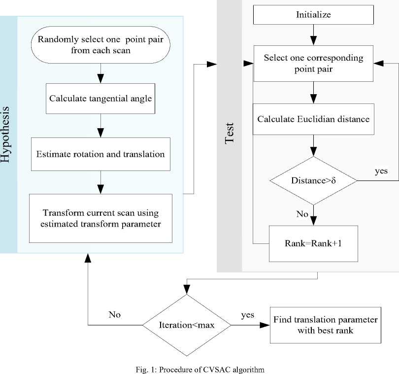
In the Test phase, considered one corresponding point of pair and calculate the Euclidian distance. After calculating Euclidian distance it checks with a threshold value (ᵟ) and then based on the condition it updates the rank and it continues till traverse all pixels. Finally, calculate the translation parameters with best rank as depicted in Fig. 1. In this way the CVSAC algorithm finds reliable scan matching parameters.

• III.    Problem Definition

The matching problem is formulated as following:

Let us consider that the used laser range sensor has an angular resolution of 0.5ᴼ. The first scan line start form 0 degree and ends at 1800 with scan line number 361. Therefor a total of 361 range measurement is achieved with an assumed measurement error of ±15mm. The laser range scan data can be modeled as:

S={ di| i=0,1,....,n di ∈ ℂ }              (1)

The measurement can be represented in phase including the margin of error ε as:

di=|ri|eje, +ε                                   (2)

where, |rj | : Measured distance at angle θ i

θi : Angular resolution Unit ×i

ε : Measurement error

In general, if the scan is taken at a position P(x, y, θ) in Cartesian coordinate, then the measurement dj can be represented as:

di=|ri|cos(θi+θ)+x

+j(|ri | sin(θi+θ)+y)+ε              (3)

Now let us consider as S ref and S scan is measured with pose P(0,0,00) and P(t ,tу,θr) respectively. We can in this case model our reference and current scan as:

S ref={d ; | i=0,1,....,n d ; ∈ ℂ }

Sscan ={dr| i=0,1,....,n d′;∈ℂ } where,

(4)         d ;=|r[|cos(θi)+j|r[ | sin(θi)+ε (5)        dr=|rr|cos(θ । +θr)+t

+j(|rг | sin(θ। +θr)+tу)+ε

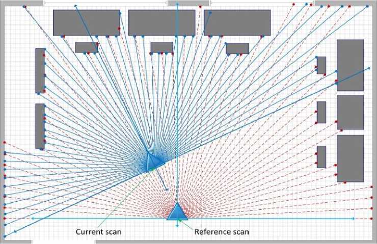
Fig. 2: Two laser scan at different position. Red (dashed) lines belongs to reference scan and blue (solid) lines represent current scan

The superscription ( ) and ( ) is used for reference scan and current scan respectively. Fig. 2 shows two scans taken at different position. Scan represented by red lines belongs to reference scan and blue lines represent the unknown current scan. Now the problem is to find the unknown parameter P(t ,ty,θr). Let us define the unknown parameter P(t ,ty,θr ) as scan matching parameter. To solve the problem, we need to find at least two corresponding point pair. Unfortunately due to the ill –conditioning of the measurement, it is difficult to find exact correspondence. Full details that will clarify the problem of finding the corresponding vector are discussed below.

• IV.    Correspondence Vector SAC4.1    Corresponding Point

Sufficient clarifying details are shown in Fig. 3 which is an enlarged version of Fig. 3. If we investigate all the points (red and blue dots), there are hardly any two points pair are perfectly over lapped. Fortunately we have one pair (red transparent circle) which perfectly overlapped. Nevertheless this pair is not a good choice as corresponding point pair. The reason behind this is explained in Fig. 4.

In another related work [22], suggests that instead of finding exactly two position pair, we can find one position pair and calculate tangential angle vector between the found measured position pair and each following measured position. But this does not completely solve the problem in every case. This is pictorially illustrated in Fig. 4.

Consecutive scan lines r^ and r2 from reference scan are measuring point PL and P2 which fit into the same plane of a fixed object-1.We chose scan lines r and r2 from current scan in such a way that at least one of them overlaps with reference scan. In this case PL is the common point measured by each of the laser scan S ref and S ref .

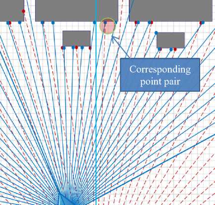
Fig. 3: Enlarged version of Fig. 2 showing the corresponding point pair

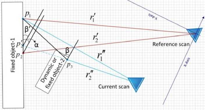
Fig. 4: Two laser scan consist of two scan line each showing the condition arise due to fixed or dynamic object appear as an obstacle in current scan

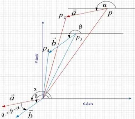
Fig. 5: P and P are two points in reference scan creating tangential angle α. P and P are their counterpart taken from current scan creating tangential angle β. θ is the estimated rotation between them

Measurement of tangential angle vector is illustrated in Fig. 4. The point P3 is measured by scan line r2 which fit into the plane of object-2. As P 7 and P3 are not on the same plane, then the tangential angle with preceding point will also be different. We can see it in Fig. 4 that β and β are not equal. Here β is measured by extending r2 up to the plane where P_L and P 7 exist. We denote this point as P2 . Consequently, P_L and corresponding tangential angle vector from reference and current scan cannot be taken as a corresponding vector. Therefore this method needs an iterative search to find the best matching pair which does not suffer from this bewildering condition. Fig. 5 geometrically illustrates the determination of the angle vector θ_r.

• 4.2    Corresponding Vector

• 4.3    Consensus Ranking System

Let us consider a case where one reference scan line r i have a tangential angle vector α with its next adjacent scan line r i+1 . Similarly we chose its corresponding current scan line r " having tangential angle β from its adjacent. These two features (r [ ,α) and (r " ,α) are defined as a corresponding vector pair. Now, our matching parameter can be estimated as:

θr=β-α

t =|r [ |cosθi-|rj"|cos(θi+θr) tу=|r;|sinθi-|rr|sin(θi +θr)

Hypothesis Step:

• •    Randomly select one point from S scan and one point from S ref

• •    Assume these two are the same point measured in both scan

• •    Find tangential angle vector of each point from its followed point

• •    Calculate θ_r using equation (6)

• •    Rotate S scan with an angle θ_r

• •    Calculate t and t

• •    Transform S to S^̂    using transform parameter

P(t ,tу,θr)

Testing Step:

Calculate the Ranking according to following equation:

R(Sref;Ŝscan)=∑i^i ρ(rc,r " )                   (7)

where, R∶ Consensus Ranking System r : A range measurement of Ŝ rс ∶ Corresponding point in S ref with rj"

ẟ ∶ Threshold

Step-3: This is the last step and we did the same thing as in step-2. The only difference is that in this case we apply the CVSAC algorithm on to the whole data and Δ 9 is chosen as 0.05^o.

Selection of corresponding points is illustratively explained in Fig. 6.

In practice, all the point does not exactly correspond and therefore we apply the consensus ranking system to achieve the best match using equation 6. We observe that a threshold of 45mm~100mm works well. If a very low threshold is selected, then the scan matching will suffers from the intrinsic measurement error of the SICK laser sensor on the other hand, if we select an arbitrarily high threshold, the matching result will contain many non-corresponding outliers. This will be true even if we chose the best corresponding pair.

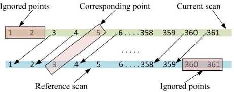
Fig. 6: P(5) from current scan and P(3) from reference are considered as corresponding point. So there preceding and following points also correspond to each other respectively

• V.    Speedup Schemes

Scan matching parameter estimated by above version of CVSAC is reasonably reliable and eliminate the extra step of finding optimal parameter using ICP explained in [5]. However, our algorithm is too slow to apply real time mobile robot pose estimation. Because the computational complexity of corresponding point search is O(n2). Therefore we introduce some speedup scheme which improves the run time dramatically without trading off the quality of the output. Even we observe that it improve the result a bit. The scheme consists of three steps:

Step-1: Instead of applying CVSAC algorithm on to the whole laser scan point we have taken an average of sixteen consecutive points each of 8^o and apply CVSAC. From this step we only extract the approximate rotation θ_r.

Step-2: This step consist of two fold filtering of data. First, we apply CVSAC algorithm only on to the even (or odd) number of laser scan point. Secondly, consensus ranking is applied on to those corresponding vector which produce a translational angle in the range of θ_r ± Δθ. We chose Δθ as 2.5^o and θ_r is taken from previous step. Again from this step we only extract the rotational angle θ_rto apply in the next step.

• VI.    Experimental Result

We performed an experiment using two raw laser scan data in a dynamic environment. In each case of experiment SICK LMS-291 laser sensor was configured as 0.5ᴼ angular resolution with 180ᴼ FOV. Fig. 7 shows tow scan plotted before matching and Fig. 8 shows two scan before matching (cyan dot represent reference scan and blue dot represent current scan. We also compare the result with ground truth in every instance. Ground truth data are collected from the measurement by hand. We tabulate two such experiment results quantitatively in Table 1.

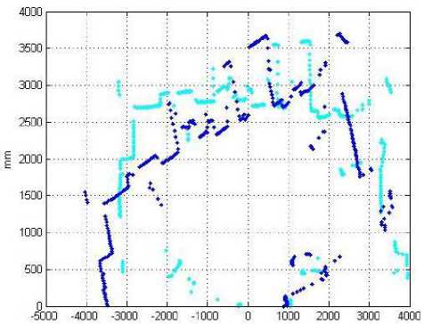
Fig. 7: Two laser scan at different position before matching

If we compare Fig. 7 and Fig. 8, we will observe that the Fast CVSAC algorithm works well in view of the processing times of 0.693 and 0.72 for each respective units of tx, ty and θr. It is instructive to note that in Fig. 8, most of the selected feature point of the dynamic cluttered environment were correctly matched which signifies that the fast CVSAC algorithm will be able to work well in even environments that does not contain sharp matching features. For robots and other intelligent machines to function well, it is quintessential that they cope with office like environment and in other environment without orthogonal and rectilinear walls that could be used to immediately compute points of references; and they must do so in fast and in real time too. Results of our fast CVSAC method promise a speedier alternative to that of dead-reckoning through the use of odometer. Also, it promises an alternative worthy of further exploration if we have an environment with only one or no matching point in a current-robot scan and its associated reference scan.

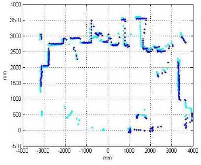
Fig. 8: Two laser scan at different position after matching

Table 1: Comparison of result with ground truth

		Measured (mm)	Result (mm)	Error (%)	Process Time(s)
a	tx	-480	-472	1. 67	0.69
	ty	400	405	-1. 25
	Or	19.8	19. 93	0. 66
b	tx	130	134.9	3. 76	0.72
	ty	240	236	1. 66
	Or	- 19.6	- 19. 65	0. 25

• VII.    Conclusion

In this paper we proposed a scan matching algorithm for robot pose estimation. Our proposed algorithm is based on CVSAC. This method does not require any feature extraction and no initial position for matching. The version of our CVSAC algorithm employs the consensus in Cartesian coordinate. We improve the high cost of testing step by averaging and subsampling the data. Our experiment shows good positive result.

However, our algorithm needs some heuristic parameter as matching criteria. These values need to be tested under different environment. Future work has to be done to select these values automatically depending upon the environment. We also want to apply this algorithm in SLAM as a future work.

Acknowledgments

The authors would link to thank the anonymous reviewers for their valuable suggestions to improve the overall quality of paper.