Leveraging Sensitivity Analysis for Configurable Kafka Clusters: A Multi-objective Model to Minimize Latency

Published Online on August 8, 2025 by MECS Press

The widespread use of Internet of Things (IoT) devices, sensors, and wearable sensing technologies has introduced new demands on real-time data processing infrastructures. Apache Kafka, a distributed event streaming platform, has become a key component in these infrastructures due to its high-throughput, fault-tolerant design [1]. However, Kafka's extensive configuration flexibility introduces significant uncertainty into system performance, particularly with regard to end-to-end latency, defined as the time taken between a producer sending data and a consumer receiving it.

Despite its importance, selecting an optimal Kafka configuration remains a challenging problem. The challenge involves dynamically adjusting the configuration to prevent overloading, and minimize costs while maintaining high availability and low latency [2].

Existing studies often focus on improving a single performance metric such as latency or robustness, overlooking the influence of latent interactions among configuration parameters and the system's sensitivity to local value changes. Consequently, this can lead in suboptimal or fragile configurations that do not generalize well in real-world deployment scenarios.

The goal of this research is to design a multi-objective model that optimizes Kafka configuration to minimize end-to-end latency while quantifies independent parameter influence, interaction effects and sensitivity to local parameter changes.

The novelty of our contribution is a formalized optimization model that integrates global and local sensitivity indices (Morris µ, Sobol, DLOR) to execute Kafka configuration tuning to prevent overloading while maintaining high availability and low latency of Kafka cluster. An adaptive optimization strategy that combines gradient-based and derivative-free algorithms to overcome local minima and nonlinearity challenges in high-dimensional parameter spaces. A validation through real-time Kafka streaming experiments, using a dataset generated from an IoT device (Hobo MX-100), with cross-verification using a trained XGBRegressor model.

This paper is structured as follows: following this Introduction and Literature Review, the Materials and Methods section provides the formal definition for the proposed multi-objective model. The Data Collection and Experimental Study section includes Kafka cluster configuration descriptions needed for this modelling. The Results and Discussion includes the detailed practical outcomes of these tests. Finally, the Conclusions section outlines the recommendations drawn from this research.

2.    Related Works

The researchers are studying models and methods to ensure the efficiency of Apache Kafka cluster configuration when integrated into the ingestion layer of system architectures. For example, in [3], a model for Kafka cluster configuration is proposed, consisting of three subsystems in series: a producer group, an Apache Kafka cluster, and a consumer group, each containing three parallel units operating under a 1-out-of-3 strategy. The developed model has been proven to improve the system's ability to handle streaming data failures.

In [4], Apache Kafka was used as the backbone of the data ingestion layer to manage high-throughput data streams in real time for an Internet banking system. The Kafka cluster was configured with multiple producers and consumers, ensuring scalability by dynamically adjusting the data ingestion rate based on the number of active producers, making it suitable for high-velocity Internet banking data.

In [5], a solution is proposed that model’s consumer provisioning as a two-dimensional bin packing problem and addresses the challenge of blocking synchronization, which affects high-percentile latency.

In our view, the solutions in [3-5] focus on single-objective optimization (e.g., minimizing latency or improving robustness). This can result in configurations that optimize one metric while ignoring other critical and sensitive configuration parameters.

Predictive maintenance (PDM) has emerged as a vital application within the IoT ecosystem, which includes Apache Kafka clusters for high-throughput, fault-tolerant data ingestion from multiple IoT sensors and producers. Machine Learning and Deep Learning pipelines are widely used in PDM architectures [6]. In [7], an end-to-end architecture is proposed for real-time predictive maintenance in IoT settings. The design integrates modern tools for data processing, machine learning lifecycle management, and performance monitoring. In [8], a Principal Component Analysis (PCA) is incorporated into a framework created to predict Kafka's workload over time. PCA was applied to eliminate variables related to Kafka's resource utilization by focusing on the most significant factors influencing cluster performance.

The reviewed models in [6-7] do not address the problem of optimizing Kafka cluster latency through configuration parameter tuning. The PCA technique used in [8] identifies parameters that vary the most in the input space, but high PCA scores do not necessarily imply a causal impact on latency. Therefore, to achieve the goal of the current study, we conduct a sensitivity analysis to measure the influence of configuration parameters on the objective function.

Sensitivity analysis is a widely used technique to understand how variations in input parameters influence the output of a model or system. In [9], a four-stage sensitivity analysis framework was proposed that integrates meta-modeling with the Morris and Sobol methods to identify significant factors influencing annual energy consumption while reducing computational costs. In [10], the impact of important features was identified using sensitivity analysis methods — Morris, Sobol, Directional Local Optimal Response (DLOR), and Fourier Amplitude Sensitivity Test (FAST). The experimental part involved evaluating the accuracy of each method by comparing the performance of a CNN model that included features selected by each method. The conclusions stated that Sobol and Morris demonstrated superior performance.

In [11], an approach was proposed to simplify the estimation of Sobol indices and complement them with the calculation of Shapley indices. Unlike the traditional approach, which first estimates first-order indices and then derives total indices, this study introduced a less computationally expensive method. In this approach, total indices are estimated first as the global effects of input combinations, and the remaining Sobol indices are then obtained through linear transformations.

In [12], global sensitivity analysis using the Sobol method was applied to rank parameters in the life cycle assessment of manufacturing technologies, allowing practitioners to focus data collection efforts on the most critical parameters. The study highlights the importance of carefully selecting and applying probabilistic values while performing sensitivity analysis.

In the current research, following the conclusions from [10] on the efficiency of the Morris and Sobol methods, we apply them to measure the impact on Kafka latency caused by two factors: 1) interactions between parameters (measured by the Morris method); and 2) independent, direct parameter influence. Since the same parameter may have different impacts depending on Kafka’s sensitivity to changes in its value, we include the DLOR method in the model as well. Following the conclusions from [11], we calculate only the first Sobol index to keep the model computationally efficient. To avoid the influence of initial dataset uncertainty on the sensitivity analysis results, as noted in [12], we test the proposed multi-objective model against Kafka end-to-end latency predicted by a trained XGBRegressor model. The XGBRegressor model is selected for verification purposes, as its XGBoost algorithm is designed to approximate non-linear datasets; XGBoost does not assume smoothness or differentiability of the input-output relationship, making it robust for noisy or discrete problems [13].

3.    Materials and Methods

Let L(X) represent the latency of Kafka cluster and X i=i^ = {x i } , is a set of n independent parameters of a Kaka cluster. The total variance in L(X) , decomposed by inputs is

Var(L(X) ) = X^! V[ + Zi

^ = VarXiJEx~iJ(f(X)IXi,Xj)) -Vi-Vj(3)

where V 1,2,…,N is interaction involving all features in the set X .

The first order Sobol Index estimates how much of the output variance in L(X) is due to input x i alone is [14]:

si =~^

¹     Var(Y)

The Morris method measure sensitivity of the output using two metrics: µ i is the mean absolute elementary effect, showing the overall importance of parameter x i ; σ is the standard deviation of effects, which indicates interactions between x i and other parameters [15]. The formula for Morris µ i is

1Л=^Г=М

where d{ is the elementary effect of input parameter xi, in the r-th iteration dr =

f(x ^r +^e [ )-f(x ^r )

△

where x^r is a random sampled vector in the r -th iterations. △ e_i is the unit vector to modify only x i . . △ is a step in search grid.

Directional Local Optimal Response (DLOR) approximates the partial derivative of the model output with respect to the input at each point [16]:

DLOR i =

f(X i +£)-f(X i) l dX i I

where £ is a learning rate, fixed or from uniform distribution in case of missing prior knowledge. DLOR i focuses on local sensitivity because the gradient is computed close to x i measuring how sensitive the output is to a small perturbation near x i .

Our multi-objective model aims to find a configuration X that minimizes Kafka latency L(X) according to equation (8) but considering the combined effect from independent influence of parameter x i with the sensitivity of latency to the changes in value of x i (9) and the combined effect from influence of parameter x i though interactions with other parameters with the sensitivity of latency to the changes in value of x i (10)

L(X) ^ min(8)

Zi=iSi(XrDLORi(X)(9)

Zi=i^(XrDLORi(X)(10)

By adding equations (9) and (10) as penalty terms to equation (8) we designed the multi-objective model:

L(X) - a’ • maxXi=1Si(X) • DLORi(X) - P • maxXi=1Pi(X) • DLORi(X) ^ min          (11)

with parameters constraints: X_i E [a_i,b_i],V_iE {1, ^,n) , a',ft' - adjusted weighs to balance the contribution of independent influence (9) and the influence through interactions with other parameters (10).

The magnitude of weights’ adjustment is estimated with Spearman’s rank correlation coefficient that measures the monotonic relationship between two variables [17]:

Spearman’s rank correlation coefficient (P s ^) between Sobol S i (X) and Morris p i (X) determines how much the local sensitivity captured by Morris aligns with the global sensitivity captured by Sobol:

_ . _ 6Z P=i (R(Si(X))-R(^i(X))²

^Ps №              n(n ² -1)

where R(S i (X), R(µ i (X) represent the ranks of pair Sobol S i (X) and Morris µ i (X) indices.

Spearman’s rank correlation coefficient ( p^dlor ) between Morris p(X and DLOR i (X) determines how well the linear component of sensitivity DLOR aligns well with the local effects identified by Morris:

6S F=i (R(^i(X)-R(DL0R(X)))^{2 P}^^{,dlor    1}              n(n 2 — 1)

where R(µ i (X), R(DLOR i (X) represents the ranks of pair Morris µ i (X) and DLOR i (X) and indices.

When Spearman’s rank correlation between two sensitivity indices is high (ρ ≤ 0.7), the information captured by both indices overlaps. This leads to an over-penalization of the objective function equation (8), and therefore, the weights α, β must be reduced. A moderate correlation (0.3 ≤ ρ<0.7) indicates partial overlap, so slightly reducing the weights helps balance the contributions of terms (9) and (10) in equation (11). A low correlation (ρ<0.3) means that the indices capture independent aspects of sensitivity in the Kafka configuration’s impact on Kafka cluster latency, and thus, no weight adjust is needed.

To solve the multi-objective design model (11), both gradient-based and derivative-free optimization algorithms are considered:

The Limited-memory Broyden–Fletcher–Goldfarb–Shanno with Bounds (L-BFGS-B) handles optimization problems for large datasets (number of features more than 100) by approximating the inverse Hessian matrix (H i ):

xl+i =xt- aiHiVf(Xi)                                       (14)

where Vf(X [ ) is a gradient at i-point; a i is a step size.

L-BFGS-B enforces bounds on each point a_i< x_i< b_i by projecting gradients when x i reaches the boundary of the feasible region. It typically finds solutions near the center of the feasible regions, avoiding solutions at boundary extremes unless the gradient or Hessian explicitly guides it there [18].

Sequential Least Squares Programming (SLSQP) is an iterative optimization algorithm where each iteration solves a quadratic programming problem (QP) to generate a search direction d:

mini dT H^d + ^f(xi)Td subject to:

Vh(xi)Td + h(xi) = 0

Vg(xt)Td + g(xt) > 0

where H_i denotes the approximate Hessain matrix of the Lagrangian function L(x_i, X_i,p_i ) with respect to x. ,X_i, p_i are the Lagrange multipliers. After solving problem QP, the line search method is used to determine a suitable step length, it behaves more conservative compared to SLSQP as it uses local quadratic models with constraints (even if none are set). The complexity of QP solvers grows with the number of variables and constraints, making the method practical for moderate problem sizes [19].

Trust-Region Method (Trust-constr) is a gradient-based optimization algorithm that, at each iteration, solves a local quadratic approximation of the objective function:

mi(d) = f(xi)+ Vf(xi)Td + ldTHid (18)

where f(x_i) is a current function value, Vf(x_i) is a gradient at X i , H_i denotes the approximation to the Hessain matrix of f at x i , d is the proposed step direction from x i . The step d is accepted only if it is improved the ratio between actual and modeled reductions:

ftxj-ftxj+d) m t (0)—m t (d)

Trust-region method is practical for moderate problem sizes [20].

The Derivative-Free Method (Powell) does not require gradients; it uses a set of search directions and performs minimizations along those directions, iteratively refining the solution. The first iteration begins with generating directions as the basis vector D⁰={e 1 ,e 2 ,.,e_n} , where e 1 =[1,0,...,0], e n =[0,0,...,1], d i =e i . For each direction d i , the function f(a) = aa² + ba + c is evaluated at three values of a 1 , a₂, a₃ and the minimum of the parabola is computed a* = —^- (Fig. 1-a ). The updated point is calculated x_n = x + a * d [ . The new direction is defined as d_n+1=x_n-x (Fig. 1-b). Directions’ list is updated by discarding the oldest direction and inserting d_n+1 at the end of the list. There calculations are repeated using updated x_n and modified direction set. The solutions produced by Powell avoids the computational complexity of Hessian approximations or solving QP subproblems [21].

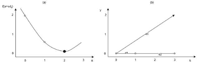
Fig.1. The parabola through the three sampled points along the y- direction with the analytical minimum at a * = 2 (a); the resulting new direction di (b)

The Nelder-Mead algorithm is a derivative-free method for minimizing a real-valued function f(x) assumes that iteration k begins by ordering and labeling vertices x]^, ...,x(2± , such that

f(k) ^ f(k) ^      f(k)

^f 1    — ^f 2    — ’” — J n+1

Compute the centroid x_c = E "= ₁x_i/n of the n best points; reflects worst point: x_r = x_c + p(x_c — x_n+1) and evaluates f r =f(x r ) . If f 1 < f_r< f_n, accepts x_r and terminates the iteration. If f 1 > f_r, calculates the expansion point x_e = x_c + A(x_r — x^ and evaluates f_e=f(x_e) . If f_e <  f_r, accepts x_e and terminates the iteration; otherwise accepts x_r and terminates the iteration. If f_n—f_r< f_n+1, performs an outside contraction by calculating x_k = x_c + %(x_r — x_c) and evaluates f_k=f(x_k) . If f_k< f_r , accepts x_k and terminates the iteration; otherwise perform a shrink. If f_r >  f_n+1, performs an inside construction x_kk = x_c — %(x_c — x_n+1) and evaluates f_kk=f(x_kk) . If f_kk< f_n+1, accepts x kk and terminates the iteration; otherwise perform a shrink. The shrink all points to the best V [ = x 1 + o(x_l — x 1 ), i=2, ..,n+1 . The unordered vertices of the simplex at the next iteration consist of x 1 ,v₂,.,v_n+1 . The effects of reflection (p=1), expansion (a=2), contraction (γ=0.5) and shrink (σ=0.5) in two dimensions are shown on Figure 2 and visually evident that the simplex shape undergoes a change. Unlike Powell, which searches along fixed directions, Nelder-Mead is less sensitive to noise in the dataset. This makes it particularly suitable for problems where objective function evaluations are noisy [22].

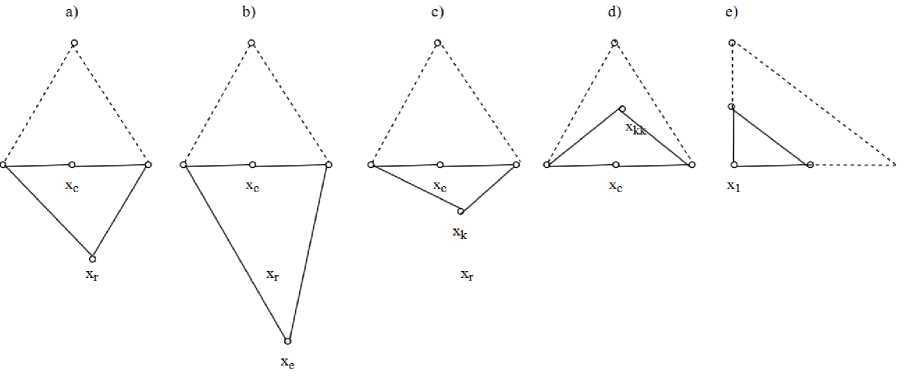
Fig.2. Nelder–Mead simplices after a reflection (a) and an expansion step (b). An outside contraction (c), an inside contraction (d), and a shrink (σ). The original simplex is shown with a dashed line

The effectiveness of the optimization algorithms listed above depends on the nature of the relationship between the input features X and the target feature L(X) in the dataset. Therefore, we propose an adaptive optimization strategy that combines gradient-based and derivative-free optimization method, aiming to select the optimal method based on two criteria:

• •    The difference between the latency calculated for the optimal configuration using equation (11) and the latency predicted by the XGBRegressor model for the same configuration is less than 1%.

• •    The minimum time complexity of the optimization method, assessed by the number of iterations required to complete the search.

To describe constraints Xi £ [a , , b , ] for model (11) each Kafka cluster parameter to be defined per notation:

where N is a name of the parameter. S is a set of state S t=iN = {s , } expressed as linguistic terms. I(S) is an interval of values for each state s , £ S.

Algorithm 1 describes in pseudocode the steps to implement the designed model (11). The input parameters’ list includes the constraints x , £ [a , , b j ],V , e {1,..., n}, denoted as “bounds” and associated with Kafka cluster test scenarios, denoted as “problem_definitions”; a list of optimization algorithm, denoted as “methods”, a trained machine learning model to rank the result of optimization algorithms. The selected for Algorithm1 machine learning model for the regression problem must be validated with metrics:

The proportion of variance in the independent features X is explained by the trained model:

R2 = 1 - SSres sstot

Where SS_res - sum of squared residuals (errors), SS_tot - total sum of squares (variance of a target variable L ).

The model predictive accuracy:

MSE^^Lt-Lty                         (23)

where L i - value of a target variable L in the collected dataset, L , - a predicted value of a target variable L in the collected dataset.

The algorithm output is a list of ranked optimization results denoted as “rankedresults”. Default values for weights α and β from equation (11) are set to 1.

Algorithm1. Pseudocode for an adaptive optimization strategy for Kafka cluster configuration

Input : problem_definitions = [{“bounds 1 ”:[[],..[]]},…,{ “bounds 5 ”:[[],..[]]}]; methods, model.

Output : rankedresults.

Initialization : α = 1; β = 1; resultslist = []; rankedresults=[].

• 1    FOR each problem in problem_definitions:

• 2    FOR each method in methods:

• 3      moris_sampling = sample(problem)

• 4       morris.mu= analyze(problem, moris_values, model.predict(moris_sampling), conf_level=0.95)

• 5       sobol.sampling = saltelli.sample(problem)

• 6       sobol= sobol.analyze(problem, model.predict(sobol_sampling))

• 7       dlor_sampling = latin.sample(problem)

• 8       dlor = dlor_sensitivity (problem, model.predict(dlor_sampling))

• 9       morris.mu.scaled=(1-min(morris.mu))/(max(morris.mu))- min(morris.mu))

• 10      dlor.scaled=(1-min(dlor))/(max(dlor))- min(dlor))

• 11      ρs,µ = calculate_spearman(sobol, morris.mu.scaled)

• 12      ρµ,dlor= calculate_spearman(morris.mu.scaled, dlor.scaled)

• 13     IF (0.7 < ps,^) THEN a' = a(1 - p_s,y ENDIF

• 14     IF (0.3 < ps,^< 0.7) THEN a' = a(1 - 0.5 • p_s^) ENDIF

• 15     IF (ps,^ < 0.3) THEN a' = a ENDIF

• 16     IF (0.7 < p^.dlor) THEN ^' = p(1 - P^dlor) ENDIF

• 17     IF (0.3 < p^dlor< 0.7) THEN 0’ = 0(1 - 0.5 • p^_DLOR) ENDIF

• 18     IF (p^dlor< 0.3) THEN 0’ = 0 ENDIF

• 19      results = minimize(objective_value, x0, args=(scaled_mu, scaled_dlor, sobol_cal['S1‘], a', 0', method),

• 20      bounds=problem['bounds'], method=method, options=options)

• 21      resultslist.append([method, cal_latency, cal_configuration, num_iterations])

• 22    ENDFOR

• 23    EndFOR

• 24    FOR each result in resultslist:

• 25   pred_latency= model,predict(result. cal_configuration)

• 26   errorscore= abs((result. cal_configuration - pred_latency)/ pred_latency)

• 27   ranklist.append[(result, errorscore, result. num_iterations)]

• 28    EndFOR

• 29    rankedresults = sort(ranklist by (errorscore, num_iterations))

4.    Experiments 4.1.    Data Collection and Experiments Preparation

In Algorithm 1, lines 3–8 perform sampling, modeling, and sensitivity analysis for each scenario defined by the given constraints. In lines 9–10, the calculated values of the DLOR and Morris indices are scaled to make them comparable; Sobol indices are already in the range [0..1], so additional scaling is not required. In lines 11-12 Spearman correlation coefficient is calculated according to (12-13). In lines 13-18: α, β weights of equation (11) are adjusted to prevent over-or under-penalization of a target variable L(X). In lines 19-20, a general-purpose optimization function, “minimize” from the scipy.optimize library is called. The parameters passed to it includes: the custom-developed by us function “objective_value” that implements equation (11); x0, the initial configuration randomly selected from the “bounds” using uniform distribution; scaled DLOR, Morris and Sobol indices; the adjusted weights; and a search method from the predefined methods list. In line 21, the Kafka cluster configuration found by the completed optimization search (denoted as cal_configuration), the corresponding latency (cal_latency), and the number of iterations required are added to results_list. In lines 24–28, for each configuration in results_list, the predicted latency is obtained using the given machine learning model. The percentage latency difference is then calculated, denoted as “errorscore” and, along with the number of iterations, stored in a list for subsequent ranking. In line 29, ranking is applied based on the keys “errorscore” and “num_iterations”. The Kafka cluster configuration selected for output is the one with rank one.

To collect a dataset for multi-objective optimization problem (11) we designed scenarios to test different Kafka cluster characteristics:

• •    A scenario to measure a Kafka cluster latency with high throughput emphasis with durability.

• •    A scenario to measure a Kafka cluster latency with low latency and average throughput.

• •    A scenario to measure a Kafka cluster latency with a balanced throughput and latency with fault tolerance.

• •    A scenario to measure a Kafka cluster latency with a stress test.

• •    A scenario to measure a Kafka cluster latency with a high fetch size for Bulk Processing.

The dataset with Kafka cluster performance in the defined scenarios 1-5 is collected as a result of the system tests with streaming event data through the steps 1.1-1.4 (Fig. 3).

Fig.3. Step to collect a dataset with kafka cluster performance

To complete subprocess 1.1 we selected a telemetry data from IoT device of type "Hobo MX-100” which is a temperature data logger, a single message size is 387 bytes is sent every second.

To completed subprocess 1.2-1.3 the states and bounds of Apache Kafka configuration parameters X={x 1 ,...,xn} were described according to a notation (21) and specified in Table 1. The specific value of each parameter for the scenarios 1-5 is defined in Table 2.

The dataset, consisting of 1000 observations (Table 3), was received after running 200 times each scenario with corresponding configuration.

The experimental study will be conducted on a system with processor 11th Gen Intel(R) Core(TM) i7-1185G7. Kafka parameters configurations. The implementation of the algorithms 'L-BFGS-B','SLSQP'; 'Trust-constr', 'Powell', 'Nelder-Mead' are from the Python scipy.optimize library.

• 4.2.    Experiments Results and Discussions

The XGBRegressor model was trained on 67% of the collected dataset D and validated on the remaining 33%. The resulting R² score of 0.83 indicates that the model captures the majority of the variance in both the input parameters X and the target feature Latency . A mean squared error (MSE) of 0.09 demonstrates the model’s high predictive accuracy (Fig. 4).

Table 1. Kafka cluster configuration parameters description

Name of parameter	Parameter description	Set of states	Set of values
acks	level of acknowledgment required from the leader-server for producers	none, leader, all	0,1,”all”
batch.size	the maximum producer batch size in bytes	small, moderate, large	[1KB..8KB],(8KB..16KB],( 16KB.. 32KB]
linger.ms	Time the producer will collect event data to form a batch	none, default, high	0,[1..50),[50..100]
compression type	the message compression type	enable, disable	“none”,“gzip”
buffer.memory	the total amount of memory the producer can use for buffering	small, default, large	[1MB..8MB],(8MB..50MB],(50MB ..96MB]
max.inflight.requests.per.co nnect	the maximum number of unacknowledged requests that can be sent to the server on one connection.	single, moderate, high	1,(2..5],(5..15]
socket.receive.buffer.bytes	the size of the network socket buffer for receiving data	small, default, large	[100KB..500KB],(500KB..1MB),[1 MB..2MB]
log.flush.interval.ms	the maximum time, that a message can remain in the log buffer before it is flushed to disk	frequent, less frequent, not frequent	[0..100),[100..500),[500..1000]
max.poll.records	the maximum number of records that a Kafka consumer can handle in one call to the poll() method	small, moderate, large	[100..300],(300..500],(500..2000]
fetch.min.bytes	minimum number of bytes that must be copied to the disk of the leaderserver before becoming available for Kafka consumers to fetch	frequent, less frequent, not frequent	[1KB..100KB],(100KB..500KB],(5 00KB..1MB]
retries.config	the number of times the producer will retry sending	low latency, balance, strong reliability	[0..2],[3..5],(5..10]

Table 2. Kafka cluster configuration parameters state for the scenarios 1-5

Name of parameter	Scenario 1	Scenario 2	Scenario 3	Scenario4	Scenario 5
acks	all	leader	all	none	all
batch.size	large	small	moderate	large	large
linger.ms	high	none	default	none	high
compression type	enable	disable	enable	disable	enable
buffer.memory	large	default	default	small	large
max.inflight.requests.per.connect	moderate	single	moderate	high	moderate
socket.receive.buffer.bytes	large	small	small	small	large
log.flush.interval.ms	less frequent	frequent	less frequent	frequent	not frequent
max.poll.records	large	small	small	large	large
fetch.min.bytes	less frequent	frequent	less frequent	frequent	not frequent
retries.config	strong reliability	low latency	balance	strong reliability	balance

Table 3. Kafka cluster performance dataset for an adaptive optimization strategy for Kafka cluster configuration

Target class names	Observations	Features	Machine learning task	Missing values, Y/N?	Duplicated values in column, Y/N?
Latency, L	1000	11	Regression	N	Y

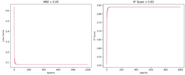
Fig.4. The results of the validation of XGBRegressor model

The results of the sensitivity analysis, based on the computed sensitivity scores, are presented in Tables 4–8. A “+” sign indicates a notable influence, defined where the sensitivity value exceeds 0.1. An analytical analysis of the sensitivity indices is summarized as:

• •    Each input parameter has a different degree of influence driven by independent impact, impact though

interactions or impact as a result its value is change around some point.

• •    The combined effect of parameter x i through interactions with other parameters dominates over both its

independent influence and its sensitivity to local value changes.

Table 4. Sensitivity scores of parameters in configuration for scenario 1. Spearman’s correlation ρ S,µ = 0.84; ρ µ,DLOR = 0.5

Parameter	Morris µ	Sobol first index	DLOR	Influence through interactions	Influence independently	Local sensitivity
linger.ms	0.08	0.00	0.00	-	-	-
batch.size	0.16	0.01	0.00	+	-	-
buffer.memory	0.01	0.00	0.00	-	-	-
max.inflight.requests.per.connect	0.08	0.00	0.09	+	-	+
retries.config	1.00	0.97	1.00	+	+	+
max.poll.records	0.06	0.00	0.00	-	-	-
fetch.min.byte	0.00	0.00	0.00	-	-	-
socket.receive.buffer.bytes	0.04	0.00	0.00	-	-
log.flush.interval.ms	0.13	0.01	0.00	+	-	-

Table 5. Sensitivity scores of parameters in configuration for scenario 2. Spearman’s correlation ρ S,µ = 0.33; ρ µ,DLOR = 0.14

Parameter	Morris µ	Sobol first index	DLOR	Influence through interactions	Influence independently	Local sensitivity
linger.ms	0.57	0.00	0.09	+	-	-
batch.size	1.00	0.34	0.00	+	+	-
buffer.memory	0.00	0.61	0.00	-	+	-
max.inflight.requests.per.connect	0.57	0.00	0.71	+	-	+
retries.config	0.68	0.02	1.00	+	-	+
max.poll.records	0.57	0.00	0.00	+	-	-
fetch.min.byte	0.66	0.02	0.00	+	-	-
socket.receive.buffer.bytes	0.57	0.00	0.00	+	-	-
log.flush.interval.ms	0.64	0.01	0.01	+	-	-

Table 6. Sensitivity scores of parameters in configuration for scenario 3. Spearman’s correlation ρ S,µ = 0.35; ρ µ,DLOR = 0.22.

Parameter	Morris µ	Sobol first index	DLOR	Influence through interactions	Influence independently	Local sensitivity
linger.ms	0.13	0.03	0.01	+	-	-
batch.size	0.43	0.03	0.00	+	-	-
buffer.memory	0.00	0.11	0.00	-	+	-
max.inflight.requests.per.connect	0.37	0.03	0.12	+	-	+
retries.config	1.00	0.71	1.00	+	+	+
max.poll.records	0.20	0.00	0.00	+	-	-
fetch.min.byte	0.37	0.03	0.00	+	-	-
socket.receive.buffer.bytes	0.25	0.00	0.00	+	-	-
log.flush.interval.ms	0.48	0.06	0.00	+	-	-

Table 7. Sensitivity scores of parameters in configuration for scenario 4. Spearman’s correlation ρ S,µ = 0.23; ρ µ,DLOR = 0.7

Parameter	Morris µ	Sobol first index	DLOR	Influence through interactions	Influence independently	Local sensitivity
linger.ms	0.13	0.00	0.00	+	-	-
batch.size	0.28	0.02	0.00	+	-	-
buffer.memory	0.00	0.03	0.00	-	-	-
max.inflight.requests.per.connect	0.40	0.03	0.16	+	-	+
retries.config	1.00	0.89	1.00	+	+	+
max.poll.records	0.09	0.03	0.00	-	-	-
fetch.min.byte	0.15	0.00	0.00	+	-	-
socket.receive.buffer.bytes	0.13	0.00	0.00	+	-	-
log.flush.interval.ms	0.14	0.00	0.00	+	-	-

Table 8. Sensitivity scores of parameters in configuration for scenario 5. Spearman’s correlation ρ S,µ = 0.98; ρ µ,DLOR = 0.3

Parameter	Morris µ	Sobol first index	DLOR	Influence through interactions	Influence independently	Local sensitivity
linger.ms	0.35	0.06	0.02	+	-	-
batch.size	0.74	0.25	0.00	+	+	-
buffer.memory	0.05	0.00	0.00	-	-	-
max.inflight.requests.per.connect	0.06	0.00	0.10	-	-	+
retries.config	0.66	0.18	1.00	+	+	+
max.poll.records	0.08	0.01	0.00	-	-	-
fetch.min.byte	0.18	0.02	0.00	+	-	-
socket.receive.buffer.bytes	0.00	0.00	0.00	-	-	-
log.flush.interval.ms	1.00	0.45	0.01	+	+	-

The calculated Spearman’s correlation coefficients (Table 9) indicate a strong alignment between the Sobol and Morris indices in Scenarios 1 and 5. However, the correlation is moderate in Scenario 2 and low in Scenarios 3 and 4. The correlation coefficients between the Morris and DLOR methods reveal moderate to low correlation, suggesting that these two methods capture distinct aspects of sensitivity and are largely unrelated. Consequently, adjustments to the weights a’ and в’ are necessary to prevent over- or under-penalization of the objective function L(X) in equation (11).

Table 9. Spearman Correlation Coefficients: ρ(S,μ) and ρ(μ,DLOR) and adjusted weights α’ and β’

Parameter	ρ S,µ	ρ µ,DLOR	a'	^
1	0.84	0.5	0.16	0.75
2	0.33	0.14	0.835	0.14
3	0.35	0.2	0.825	0.2
4	0.23	0.73	0.23	0.27
5	0.98	0.33	0.02	0.835

With PCA analysis are received a top three ranked features (Fig. 5): logflushintervalms with a contribution score of 0.42; socketreceivebufferbytes with 0.4; fetchminbyte with 0.39 impact. These features contribute the most to the variance in the input configuration space X , as identified by PCA. However, when comparing with sensitivity analysis results (Tables 4-8), the interpretation shifts: logflushintervalms shows notable influence though interactions with other parameters across all five scenarios, but its independent influence is noticeable only in scenario 5. This suggest that tuning only parameter logflushintervalms in scenarios 1-4 is unlikely to yield latency improvements. Parameters socketreceivebufferbytes, fetchminbyte have a notable influence though interactions with other parameters in scenarios 2-4, but changes in their values don’t directly impact latency in any scenario.

The search results of the designed multiple-objective model (11), obtained using optimization algorithms L-BFGS-B, SLSQP, Trust-constr, Powell, and Nelder-Mead, are presented in the “Objective latency, L(X)” column of Table 10. The number of iterations required to complete the search is shown in the “Search Iterations” column.

The XGBRegressor was run using the configurations identified through the optimization search, with the results displayed in the “Predicted latency, Lp(X)” column. The differences between the values in “Objective latency, L(X)” and “Predicted latency, Lp(X)” are calculated and expressed as percentages in the “Latency difference, %” column. The analysis of these results is as follows:

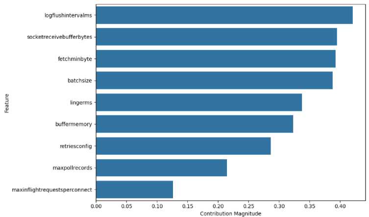
Fig.5. Kafka cluster configuration parameters, ranked with PCA

The L-BFGS-B and SLSQP methods consistently converged rapidly (within 10 iterations) across all scenarios. However, the configurations found by these algorithms did not yield optimal latency; the resulting latencies exceeded the predicted values in all scenarios.

The Trust-constr method required a moderate number of iterations (20–100) and demonstrated less than 1% difference between the objective latency L(X) and the predicted latency Lp(X) across all scenarios.

Table 10. Objective latency and time complexity for completed search for kafka cluster configuration

Scenario	Method	Objective latency, L(X)	Predicted latency, Lp(X)	Search Iterations	Latency difference, %	Search method rank
0	L-BFGS-B	367.406	355.684	10	-3.30%	n/a
0	SLSQP	367.406	355.684	10	-3.30%	n/a
0	Trust-constr	355.406	355.684	30	0.08%	1
0	Powell	355.406	355.684	301	0.08%	2
0	Nelder-Mead	355.406	355.684	408	0.08%	3
1	SLSQP	5.145	5.037	10	-2.14%	n/a
1	Trust-constr	5.010	5.037	20	0.54%	1
1	L-BFGS-B	5.145	5.037	210	-2.14%	n/a
1	Powell	5.010	5.037	264	0.54%	2
1	Nelder-Mead		5.037	10999	100.00%	3
2	L-BFGS-B	5.120	2.940	10	-74.17%	n/a
2	SLSQP	5.120	2.940	10	-74.17%	n/a
2	Trust-constr	2.930	2.940	30	0.34%	1
2	Nelder-Mead	2.930	2.940	395	0.34%	2
2	Powell	2.930	2.940	598	0.34%	3
3	L-BFGS-B	300.418	243.423	10	-23.41%	n/a
3	SLSQP	300.418	243.423	10	-23.41%	n/a
3	Trust-constr	241.418	243.423	100	0.82%	1
3	Powell	241.418	243.423	283	0.82%	2
3	Nelder-Mead	241.418	243.423	375	0.82%	3
4	L-BFGS-B	190.000	181.415	10	-4.73%	n/a
4	SLSQP	190.000	181.415	10	-4.73%	n/a
4	Trust-constr	181.192	181.415	30	0.12%	1
4	Powell	181.192	181.415	294	0.12%	2
4	Nelder-Mead	181.192	181.415	395	0.12%	3

The Powell and Nelder-Mead methods achieved similar final objective latencies to Trust-constr, with very small deviations (ranging from 0.08% to 0.82%). However, these methods required significantly more iterations (up to 598 for Powell and 397 for Nelder-Mead), indicating a trade-off between accuracy and computational efficiency. Additionally, Nelder-Mead failed to converge in Scenario 2.

In Table 10, the “Latency difference, %” for Trust-constr, Powell, and Nelder-Mead is below 1%, this matches the error rate of the machine learning model, as calculated using the MSE metric (Fig. 4).

Based on the sensitivity analysis (Tables 4-8), the optimization landscape is nonlinear and shaped by complex parameter dependencies. Since L-BFGS-B and SLSQP methods assume that the objective function has locally smooth curvature, they tend to converge prematurely to suboptimal regions, illustrated in Figure 6 by the red line, that stuck after 10 iterations at a local minimum.

Trust-constr method outperformed L-BFGS-B and SLSQP in this study because its ability to dynamically adjust the gradient step size when the predicted improvement deviates from the actual improvement. This adaptive behavior of Trust-constr helped to avoid premature convergence as illustrated in Figure 6 by the green line.

Powell and Nelder-Mead do not rely on gradient information. Instead, they explore parameter interactions through multi-point evaluations. They produced accurate results but required more iterations to complete the search.

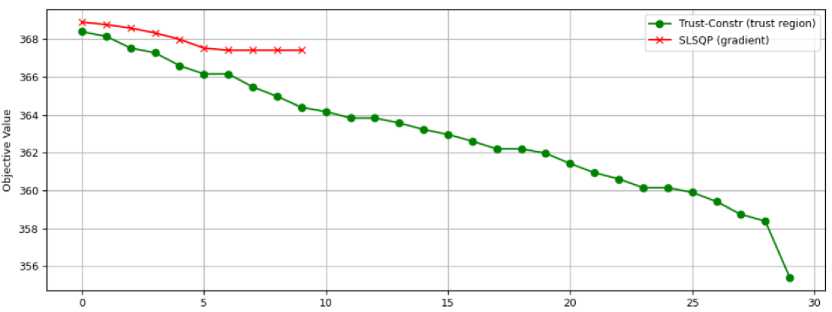
Fig.6. Gradient based optimization search by method SLSQP and gradient based with trust region search by method Trust-constr in the first scenario

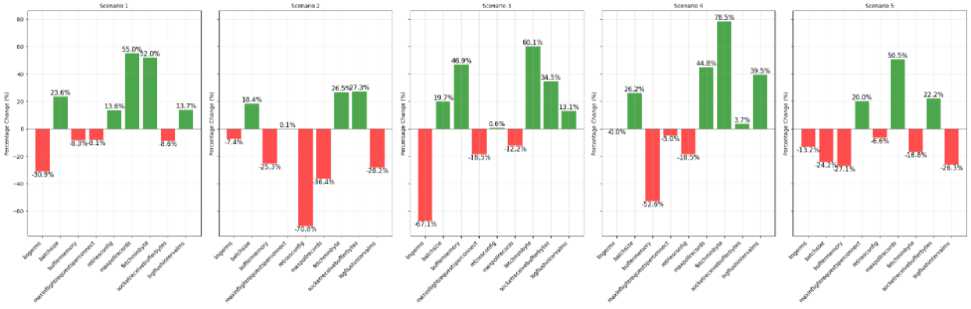
Fig.7. Percentage changes in kafka configuration parameters when optimal search is completed with algorithm trust-constr

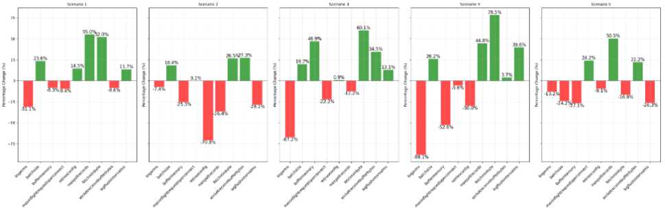
Fig.8. Percentage changes in kafka configuration parameters when optimal search is completed with algorithm nelder-mead

Figures 7-9 illustrate the percentage differences between the initial configurations and those produced by the optimization algorithms. These differences highlight how much each algorithm's solution diverged from the baseline settings. Trust-constr, Nelder-Mead, and Powell methods identified distinct configurations yet achieved comparable latency results.

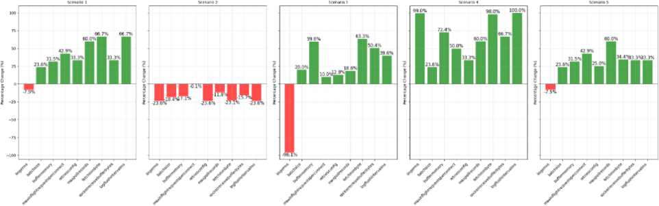
Fig.9. Percentage changes in kafka configuration parameters when optimal search is completed with algorithm powell

5.    Conclusions

In the current research, we propose a multi-objective model that optimizes Kafka configuration to minimize end-to-end latency while quantifies independent parameter influence, interaction effects and sensitivity to local parameter changes. The algorithm is designed to implement this model using an adaptive optimization strategy that combines gradient-based and derivative-free search methods. This strategy allows for a balance between convergence speed and global search capabilities, which is critical when dealing with the nonlinear parameter space characteristic of large-scale Kafka deployments.

Sensitivity analysis with Morris µ, Sobol, and DLOR indices, conducted in this study, revealed that the combined effect of Kafka cluster configuration parameters through their interactions with other parameters, dominates over both its independent influence and its sensitivity to local value changes. So, Principal Component Analysis identifies parameters that vary most within the configuration space but does not imply causality impact is unlikely to help minimize Kafka cluster latency, if used for evaluating the impact of configuration parameter on Kafka cluster latency.

The proposed multi-objective model was evaluated using five optimization search algorithms: L-BFGS-B, SLSQP, Trust-constr, Powell and Nelder-Mead. Validation of the received results was done against the predictions of a trained XGBRegressor model (R² = 0.83, MSE = 0.09) and revealed less than 1% latency difference for Trust-constr, Powell, and Nelder-Mead algorithms. This confirms the accuracy and practical reliability of the model. Gradient-based methods L-BFGS-B and SLSQP were prone to trapping in local minima due to not smoothed curvature in the objective function.

Experimental results showed that the Trust-constr, Nelder-Mead, and Powell methods identified distinct configurations yet achieved comparable latency results. Such behavior implies a level of redundancy or flexibility in configuration tuning, where alternative configurations may be selected to meet secondary objectives-such as operational constraints - without significantly impacting latency. In this context, the designed multi-objective model serves as a valuable tool to guide the configuration selection process by quantifying and incorporating such secondary objectives into the optimization landscape.

Overall, the proposed multi-objective function, validated by machine learning prediction and tested across multiple optimization strategies, offers a robust and practical tool for Kafka performance tuning.

Future work will explore how to integrate the designed multi-objective function into a dynamic optimization framework, suitable for real-time deployment and scaling scenarios.