Local Reweighted Kernel Regression

Here introduce the paper, and put a nomenclature if necessary, in a box with the same font size as the rest of the paper. The paragraphs continue from here and are only separated by headings, subheadings, images and formulae. The section headings are arranged by numbers, bold and 10 pt. Here follows further instructions for authors. Learning to fit data with noise is an important research problem in many real-world data mining applications. Kernel tricks have attracted more and more research attention recently. Fro given data set S = {( x_t , y_t )} n₌ j, the solution of the kernel learning problem is of the form

n

m (x) = ^«Л(x, x)

i = 1

* Corresponding author. E-mail address:

Where a are the coefficients to be learned from examples, while K is positive definite kernel associated with RKHS H . Recently, using multiple kernels instead of a single one can enhance the interpretability and improve performance [1]. In such cases, a convenient approach is to consider:

NN

K(x, x‘) = E cK (x, x'), s.t. E c = 1, c > 0

i = 1                                i = 1

Where N is the total number of kernels. In general, the correct number of kernels is unknown, and simultaneously determining the required number of kernels as well as estimating the associated parameters of MKL is a challenging problem [1].

For non-flat functions which comprise both the steep variations and the smooth variations, it is sometimes unsuitable to use one kernel even if a composite multiple kernel with several global bandwidths to estimate the unknown function [2]. First, the kernels are chosen prior to learning, which may be not adaptive to the characteristics of the function so that underfittings and overfittings occur frequently in the estimated function [3]. Although, the localized multiple kernel learning proposed in is adaptive to portions of high and low curvature, it is sensitive to initial parameters. Second, how to determine the number of kernels is unanswered. Finally, classical kernel regression methods exhibit a poor boundary performance [5] [6] [7].

The rest of this correspondence is organized as follows. In section 2, we proposed an iterative localized regression to deal with nonflat function regression problem. Section 3 presented regression results on numerical experiments on synthesis and real-world data sets while section 4 concludes the paper and contains remarks and other issues about future work.

• 2.    Localized reweighted regression method

  • 2.1.    Related Work

    Nadarya (1964) [8] and Watson (1964) [9] proposed to estimate m ( x ) using a kernel as a weighting function. Given the sample data set S = {( x_t , y_t )} n₌ j:

m ˆ ( x ; S )

E L Kh(x, x) yj E L Kh(x, x)

n

= Ew( x; S) y t i=1

n

Where w_i ( x ; S ) = [ E Kh ( x , x )] 1 Kh ( x , xi ) is the Nadaraya-Watson weights, such that i = 1

n

E Wj(x; s ) = 1, vx j=1

And K_h ( x ) = h ¹ K ( x / h ) is a kernel with bandwidth h .

Associating blockwise technique, we propose an improved localized kernel regression estimator which achieves automatic data-driven bandwidth selection. Suppose the initial data set S is partitioned into p

p dp such that Ebj = n [11]. For given x , if j=1

blocks denote by SS ,SS ,...,SS with length d ,d there is some block SS such that x min{xt | x e SS,} < x < max{xt | xt e SS }

Then the blockwised Nadaraya-Watson estimator is given as follows

У K. ( x , x. ) y.

m (x; SS,) = ^SS---------= У wt (x; SS,) y x                         i    xi

7 x e SS^ K h ^{( x} , x )     x e ^SS x

As thus, the localized estimator presents the unknown function m without a complicated parameters selection procedure.

• 2.2.    The new regression method

Given a dataset S = {(x;, y), x; e Rn, y e R}. Assume that m(x) e H, where H is some reproducing kernel Hilbert space called active space, with respect to the reproducing kernel K . The square norm related to the inner product by ||f||= ^ f, f   . Consider the problem, min H(m) = ^^L(y, m(x)) + AP(m)(3)

• i = 1

Where A is a positive number which balances the trade-off between fitness and smoothness; L is a loss function; P(m) = ||m||  is penalized function By the represent theory, the solution of equation (3) is [12], m (x) = £ a K (x, x )(4)

i = 1

A generalized framework of kernel is defined as

N

K ( x, x') = У cK (x, x')(5)

i = 1

Where K , i = 1,..., N are N positive definite kernels on the same input space X , and each of them being associated to a RKHS H whose elements will be denoted f and endowed with an inner product ^ •, -^. , and { c_t }_; N j are coefficients to be learned under the nonnegative and unity constraints

N

У С = 1, C i > 0,1 <  i <  N                                                         (6)

i = 1

How to determine N is an unanswered problem. For any C_t >  0 , H ‘ is the Hilbert space derived from H as follows:

H ' = { fLf e H i : f H ^ <» } c_i

Endowed with the inner product

(f, gL - =—ff, g\ici

Within this framework, H ‘ is a RKHS with kernel K ‘ = CK_i ( x , x ) , since

m (x) = (m (•), K(x, •)) H = (m o, ciKi(x, •) H,

Then, we define H as the direct sum of the RKHS H . Substituting (5) into (4), an updated equation of (2) is obtained as follows, n

m ( x) = E a K ( x, x)

i = 1

nN

=EaE cjKj(x, xi)

i=1

NnN

=E cj E aiKj(x, xi)=E mj(x) j=1     i=1

Instead of the equation (3), we convert to consider the models for j = 1,..., N ,

n

min Hj (mj) = E L (Уп mj (x )) + j (mj)

i = 1

Then, the kernel learning problem can thus be envisioned as learning a predictor belonging to a series of adaptive hypothesis space endowed with a kernel function. The forthcoming part explains how we solve this problem. Assume that a kernel function K (•, •) and corresponding reproducing kernel Hilbert space Hx are included, and then we get the initial estimator,

7 m ] ( X ) =

E 1 E x . ss Kh (X ■ xi) y EP■ Ex. SSjKh (X . X)

The residual function can be obtained,

resx (x) = m (x) — mx (x) . V = H — H/

If we have introduced t kernels {K }t , then the estimator can be updated as t        tn

Tm (x) = E rm j(x) = EE^/Kj(x, xi) j=1                j=1 i=1

And the residual function,

rest ( x) = m (x) — th (x)

If the measurements of res_t fulfilled certain thresholding criteria, here we employ 2-norm, N = t represents the number of introduced kernels and puts an end to iteration procedure. If not, considering the problem in the decreased subspace H ‘₊₁ , compute res_x = y_x — 7 m ( x_x ) and update the sample set S = {( x_x , res_x )} which can be treated as the limited of the initial data set in H_t+x .

Employing iteration, we will consider a new regression problem on the updated sample data set in a decreased subspace.

Compared with the general MKL, the first advantage is that it needs not to select weights a which will reduce much more computation burden and just need to select one kernel bandwidth at each iteration step.

Furthermore, the new method is adaptive to the local curvature variation and improves the boundary performance as a result of the introduction of blockwised Nadaraya-Watson estimate technique. At last, the number of kernels introduced will change according to real data settings based on iteration which will avoid underfitting and overfitting problem effectively.

• 2.3.    Alogorithm

The complete algorithm of Iterative Localized Kernel Reweighted Regression can be briefly described by the following steps:

• 1)    Input S , the maximum iterarion step M , threshold £ , N = 1 ;

• 2)    Initialize the pilot estimator m ( x ) = 0 , and pilot residual e = y ;

• 3)    Update the data set S = {( x _y, e _y)} n₌₁;

• 4)    Select kernel K , compute the estimator m ˆ ( x ; S ) with equation (9);

• 5)   Update the estimator m ( x ) = m ( x ) + ml ( x ; S ) ;

• 6)   Update the residuals e = y — m ( x ) , and N = N + 1 ;

• 7)    c alculate the norm of residual e .

• 3.    Experiment results

• 3.1.    Application to Simulated Data

Repeating the steps from 3) to 7), this process is continued until the norm of residual e is smaller than the pre-determined value ^£ or the iteration step ^N is larger than the pre-determined value M .

In order to select parameters, we choose 10-fold cross-validation: randomly divide the given data into ten blocks and consider the Generalized Cross Validation function is given as

GCV (0) =  £ (mij1 — m )2

Where 0 represents the set of relevant parameters, and rii ⁽ j ) is the estimator of m without the jth block samples of S .

We have conducted studies on simulated data and real-world data using the proposed method.

The test function is the mixture of Gaussian and Laplacian distributions define by i (x—2)2       q

m (x) = 2^ne 2 + T e

The number of data points for experiment is 200, and the experiment was repeated 50 times. Figure 1(a) shows the target values which were corrupted by white noise. The performance of the experiment was shown in Figure 1, in which the slender line present the true test function and the bold line represented the estimated results. Figure 1(b) represented the estimated curve using the proposed method with two step iteration which deals well with different portions with different curvature; Figure 1(c) demonstrated the standard single kernel regression based on Gaussian kernel with a global bandwidth. For this example, it can be seen that the Iterative Localized Kernel regression method achieved the better performance. Compared with the proposed method, the single kernel regression could not avoid underfitting and overfitting simultaneously and sensitive to noise at the boundary area.

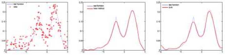
Fig. 1. The test function (slender line) and the approximation function (bold line). Figure (a) shows simulated data with white noise (SNR=20); Figure (b) shows the estimated curve using the new method; Figure (c) demonstrates the standard single kernel regression result.

• 3.2.    Application to real data: Burning Ethanol Data

  To evaluate the performance of our proposed method in practice, we analyzed the Burning Ethanol Data set. Figure 2(a) shows the data set of Brinkmann (1981) that has been analyzed extensively. The data consist of 88 a measurement from an experiment in which ethanol was burned in a single cylinder automobile test engine. Because of the nature of the experiment, the observations are not available at equally-spaced design points, and the variability is larger for low equivalence ratio.

• 4.    Conclusions and discussion

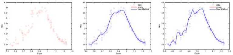
Fig. 2. Figure (a) shows Burning Ethanol Data; The blue bold lines in figure (b) and (c) show different estimated curves with two and three kernels.

As we all know, it is a difficult problem to control the pump around 0.8. Figure 2 shows the regression results with different parameters and iteration steps. The red line represents the single kernel estimator. The blue in figure 4(b)-(c) represent the estimators after two and three steps iteration with different kernel bandwidths which are determined by GCV. From the experimental results, several advantages can be drawn. First, all the estimated curves have not a spurious high-frequency feature when the equivalence ratio is around 0.8 which is the drawback other regression methods must deal with cautiously. Second, compared with [13], the proposed method is not sensitive to the pilot estimator and the kernel bandwidth selection. Finally, all the fitting results show the good boundary performance.

In this paper, we consider the kernel trick and proposed an iterative localized reweighted kernel regression method which includes two parts. At first, an improved Nadaraya-Watson estimator is introduced based on blockwised approach, which improves the classical Nadaraya-Watson estimator to be adaptive to different portions wit different curvatures; Then, considering the shortcoming of general MKR, we proposed a novel kernel selection framework during iteration procedure which avoids underfitting and overfitting effectively.

The simulation results show that the proposed method is less sensitive to noise level and pilot selection. Furthermore, experiments on simulated and real data set demonstrate that the new method is adaptive to the local curvature variation and improves boundary performance. It is easy to extend the method to other type additive noise. Kernel function plays an important role in kernel trick and can only work well in some circumstances, so, how to construct a new kernel function according to the given sample data settings is another direction we will keep up with.