Machine learning application to improve COCOMO model using neural networks

Published Online March 2018 in MECS

Every domain of our life is covered with overwhelming applications of computers now-a-days. No aspect left untouched by computers i.e. hardware and software. It is found that the prices for computer hardware has decreased in comparison of software which is continuously increasing. Software Industry annually spend the billions on the acquisition and maintenance of software [1].

Object-oriented programming, computer-aided software engineering (CASE), COTS, Agile Methodology and other technology are in use for software development, but software effort estimation has somewhere lagged behind in terms of advancements. One major resource for software product is Man-power, the effort. Estimation models first compute the effort required to complete the project, that can be further converted into dollars. The current estimation models dishearten project managers by over-estimated budget or under-estimated budget resulting into a complete failure. Various models for software cost estimation are available in market.

The most popular one is the Constructive Cost Model, or COCOMO developed by Barry Boehm [2]. The basis for COCOMO is a database of sixty-three projects created at TRW during the 1960's and 1970's and is published in Boehm's book, Software Engineering Economics. The popularity of COCOMO lies in its ease of application and its non-proprietary nature. Other models, like ESTIMACS are proprietary. In all these models the inputs and the relationships are domain specific which are fully dependent on the experts opinion. For this reason, such models tend to perform poor or even fail when their application boundaries are tried to be changed.

In such scenario, there is a need of a technique that can substitute the expert-judgement. The destined answer is Machine Learning. Data Collection, Knowledge acquisition, classification, pattern recognition and much more can be done easily and efficiently. Here we tried to apply Machine Learning to Software Engineering in Effort Estimation. Neural Network allows to model a complex set of relationship between the dependent variable and the independent variables. If we consider effort as dependent attribute and cost drivers with software size as independent entities then, neural network can be implemented as machine learning tool.

The overall objective is to design a methodology for machine learning based approach to software effort estimation using neural networks. Because current estimation models provide only marginal results within their domain specific applications otherwise, tend to fail when applied for latest development methods. The performance of proposed model based on machine-learning technique is evaluated and analyzed in comparison to the traditional models.

This proposed model uses the COCOMO data set for training phase and the Kemmerer data set for testing purposes. Then, the effectiveness of machine-learning technique to the effort estimation field is determined and post-analysis conclusion is drawn.

With this research work, we tried not only to develop a better opportunity for cost estimation but also tried to apply machine learning to software engineering.

This paper is structured into six sections as follows: Section II, discusses the background of the research work theme. Section III, covers the literature survey highlighting the various accuracy reports of COCOMO model and brings a torch on the contributions made by various researchers. Section IV, provides the experimental set-up which includes the design of proposed model and the training/testing data sets. Detailed architecture of proposed model is comprised of multiple network configurations to carry out the experiment. Section V, shows how machine learning is applied using the training data set as the means for knowledge acquisition via neural network. Then, the resulting model is tested using testing data set. The training and testing data-set are different to determine the capability of the models to generalize. In section VI displays the findings of work. The results of experiments with multiple neural networks configurations are analyzed on overall performance against actual project effort and against each other. Section VII, sums up the analysis with the conclusions made out of the entire research work.

• II.    Background

Effort estimation is all time catch for software industry when it comes to the point of accuracy. Various software developers, Engineers and reseachers contributed to this area. Multiple techniques and paradigms are already available in the industry and machine learning is one of the growing approach in this area. The stems of the current work lies in the COCOMO empirical equation and neural network technology.

The remaining section brings light on the stem and expansion of the proposed work.

• A.    Effort Estimation

A big challenge is being faced by software developers in name of effort estimation. A wide range of techniques are being employed for effort estimation like Analogy based estimation [3], estimation by expert [4], rule induction techniques [5], algorithmic techniques with empirical strategies [6], artificial neural network designed methods [7, 8, 9], decision tree based strategies [10], Bayesian network techniques [11] and fuzzy logic based estimation structures [12] and ad-hoc approach based [13].

Software Estimation Models are categorized into Algorithmic and Non Algorithmic techniques as shown in

Fig.1. which are further classified as Linear/non linear models, Discrete models, Multiplicative models, Power Function models [14].

Algorithmic models are formula based models derived from some project data. These compute effort by performing some calibration on the pre-specified formulae. Some examples are:

• a)    COCOMO model [1, 2]

• b)    Putnams’ model and SLIM [16]

• c)    Function Point Analysis (FPA) [15]

• d)    ESTIMACS

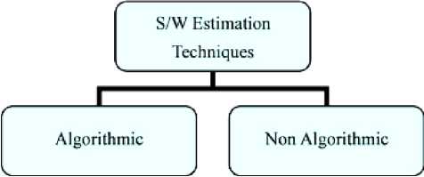
Fig.1. Software Estimation Models

The Constructive Cost Model COCOMO, was developed by Barry Boehm in the late 1970's, during his tenure at TRW, and published in 1981, Software Engineering Economics. This model is a hierarchy of three models basic, Intermediate and detailed. It is based on a study of 63 projects developed at TRW from the period of 1964 to 1979. Three development modes were defined as organic, semidetached, and embedded [2].

Initially, three development modes were defined then; calibration was made using the original 56 project database to get better accuracy. Few more projects were added to the original database resulting into the famous 63 project database. COCOMO relies on empirically derived relationships among the various cost drivers [2]. This model is popular because of the ease of its application and availability.

The basic COCOMO equations take the form:

Effort Applied,

E = a ∙ (SLOC) b           [man-months]    (1)

Development Time,

D = c ∙ (Effort Applied) d [months]      (2)

where, SLOC is the estimated number of delivered lines (expressed in thousands ) of code for project, The coefficients a, b, c and d are dependent upon the three modes of development of projects.

Non-Algorithmic models were introduced in 1990s. The inability of algorithmic methods to reason directed the path to the exploration of non-algorithmic methods. Examples are:

• a)    Case-based reasoning (CBR)

• b)    Analogy Based Estimation

• c)    Delphi Techniques

Estimation techniques are being experimented considering fusion with soft computing approach. Hodgkinson et al. [17] concluded that estimation by expert judgment performed better to regression based models. A Neuro-fuzzy approach [18], came into light considering the linguistic attributes of a fuzzy system and combining them with a neural network. Burgess et al. applied genetic programming to carry software effort estimation [19].

• B.    Machine Learning

Machine learning based effort estimation falls under non-algorithmic approach. It covers the use of neural network, genetic algorithms and CBR techniques.

The neural network paradigm grew out from the idea of imitating the human brain. Initial efforts were made by early artificial intelligence researchers. In 1958, Frank Rosenblatt defined a neural network structure called a perceptron [20]. He outlined the principles about storing the information in connecting weights. This research introduced all kind of training algorithms, supervised and unsupervised. Next milestone in the colored paradigm of neural network was the work done by John Hopfield [20]. The Defense Advanced Research Projects Agency sponsored a neural network review in 1988 and published a report on the field [21].

Neural Network is a massively parallel adaptive network of simple nonlinear computing elements called Neurons, which are intended to abstract and model some of the functionality of the human nervous system in an attempt to partially capture some of its computational strengths [22, 23, 24].

Fig.2. A basic neuron

Basic Components of a neural network as shown in fig. 2.:

• i)    neurons,

• ii)    activation function,

• iii)    signal function,

• iv)    pattern of connectivity,

• v)    activity aggregation rule,

• vi)    activation rule,

• vii)    learning rule and

viii) environment [25].

u = X WjXj     У = Ф ( ^u + b )

i = 1

where x1 ,x2, … , xn are the input signals , w1,w2, …, wn are the synaptic weights, u is the linear combiner output, b is the bias,

Φ is the activation function and y is the output signal of the neuron.

First up, a neural network is created then, it is trained which involves the modification of the weights in the connections between network layers with the objective to achieve the target output, is called learning. There are two classes of learning:   Supervised Learning and

Unsupervised Learning [23, 24].

In supervised training, both the inputs and the outputs are provided. The network then processes the inputs, compares its resulting outputs against the desired outputs and error is calculated.

In unsupervised training, the network is provided with inputs but not with desired outputs. The system itself must then decide what features it will use to group the input data [22].

Architecture of neural network: feed-forward neural network, is the architecture in which the network has no loops. Feed-back (recurrent) is an architecture in which loops occurs in the network [23, 24].

Further, Network can be a single-layered network or a multi-layered network. In single layer architecture, it consists of a single layer of output nodes, the inputs neurons are connected directly to the outputs neurons via a series of weights. But in multi layer architecture, there is an additional layer of neurons present between input and output layers. That layer is called hidden layer [23, 24]. Any number of hidden layers can be added according to the requirement of the situation and accuracy desired. In this paper we have used multiple layer feed forward neural network.

The most popular networks and the selected one in my work, is the back-propagation network. It is named after the training method used in this network. The network is a feed-forward network constructed of input layer of neurons, an output layer of neurons, and one or more hidden layers of neurons. Each neuron (or node) is defined by a transfer function.

In the case of the back-propagation network, the function usually has a sigmoid or S-shape that ranges asymptotically between zero and one. The reason for choosing the sigmoid is that the function must be continuously differentiable and should be asymptotic for infinitely large positive and negative values of the independent variables [21]. The neurons in each layer are then assigned a weighted connection to each neuron in the following layer. These connection weights are established randomly upon initialization of training and then re-calculated as the network is presented with the training patterns until the error of the output is minimized. The method that adjusts the weights is known as the

Generalized Delta Rule which is a method based on derivatives that allows for the connection weights to be adjusted to obtain the least-mean square of the error in the output [21].

Bias neurons, if used, imply provide a constant input signal to the neurons in a particular layer and relieve some of the pressure from the learning process for the connection weights.

A simple network diagram is shown in Fig. 3.

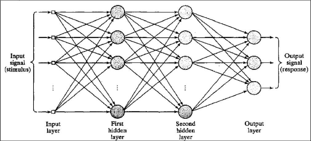
Fig.3. A Simplified Back-propagation Network

During the training process, the connection weights (and threshold values) are adjusted using the following equation [22]:

w(new) = w(old) + a * Delta(w) - output _ activation _ level where w, stands for the new and old values of the connection weight and is a constant that defines the magnitude of the effect of Delta on the weight. Delta describes a function that is proportional to the negative of the derivative of the error with respect to the connection weight and output_activation_ level is the output of the neuron.

This back-propagation of error mechanism allows the weights at all layers to be adjusted as the training process is performed, including any connections between hidden layer neurons.

A back-propagation network is capable of generalizing and feature detection because it is trained with different examples whose features become embedded in the weights of the hidden layer nodes [21]. An example of the operation of a neural network is provided by Maren and involves a neural network designed to solve an XOR classification problem.

Applications of Neural networks are in the areas of filtering, image and voice recognition, financial analysis, and.

• III.    Related Works

Although, extensive research work has been carried out in past few decades for an accurate estimation technique.

But, we are lagging behind somewhere because traditional techniques like COCOMO model are not suitable for current market trends.

MayaZaki and Mori [26]

In 1985, the accuracy of COCOMO model was reported by MayaZaki and Mori [26], in consideration of the study of 33 software projects. The MMRE was found at 165.6%.

Kemerer [27]

In 1987 Kemerer [27], in the paper entitled An Empirical Validation of Software Cost Estimation Models compared the accuracy of 4 estimation models FPA, COCOMO, SLIM, and ESTIMACS. He analyzed many COCOMO models. COCOMO Intermediate showed the least Mean Magnitude of Relative Error (MMRE). The Mean Magnitude of Relative Error (MMRE) of the 15 projects was 583.82%. Likewise, He presented project data for SLIM, ESTIMACS and FP Models.

Table I shows the effort estimate (man-month), the actual effort (man-month), and percentage MRE data of the 15 software projects using COCOMO for the effort estimation.

Kemerer used data collected from 15 completed software projects to produce results. Each model was tested for predictive capability for effort estimation. The result made was that the models require substantial calibration. He also identified the main attributes which affect software productivity [27].

Chandrasekaran and Kumar [28]

In 2012, another case study was reported while applying both COCOMO model and Function Point Analysis for the software project effort estimation by Chandrasekaran percentage MMRE (8.4%) for the COCOMO model and Kumar [28], He published the accuracy report with estimation.

Table 1. Kemerer Data-Set

DETAILS OF THE SOFTWARE PROJECTS FROM KEMERER [27]
Project No.	Estimated Effort	Actual Effort	MRE (%)
	(person month)	(person month)
1	917.56	287.00	219.71
2	151.66	82.50	83.83
3	6,182.65	1,107.30	458.35
4	558.98	86.90	543.25
5	1,344.20	336.30	299.70
6	313.36	84.00	273.05
7	234.78	23.20	911.98
8	1,165.70	130.30	794.63
9	4,248.73	116.00	3,562.70
10	180.29	72.00	150.40
11	1,520.04	258.70	487.57
12	558.12	230.70	141.82
13	1,073.47	157.00	583.74
14	629.22	246.90	154.85
15	133.94	69.90	91.62
	MMRE	583.82

Tharwon Arnuphaptrairong [29]

In 2016, Arnuphaptrairong made a literature survey to find which software effort estimation model is more accurate? He reported that Use Case Point Analysis outperforms other models with the least weighted average Mean Magnitude of Relative Error (MMRE) of 39.11%, compare to 90.38% for Function Point Analysis and 284.61% for COCOMO model. It indicates that there is still need to improve the estimation performance but the question is how.

The availability of accuracy reports tabulated in Table 2., satisfying research criteria is found to be low. Only 3 studies are made available [29] from the contributions of MayaZaki and Mori in 1985 [26], Kemerer in 1987 [27], and Chandrasekaran and Kumar in 2012 [28].

Table 2. COCOMO accuracy reports

SUMMARY OF THREE COCOMO STUDIES [29]

		Number of
S. No.	Contributor	Software project	MMRE (%)
1	MayaZaki and Mori	33	165.60
2	Kemerer Chandrasekaran and	15	583.82
3	Kumar	1	8.4
Weighted Average MMRE		284.61

Therefore other techniques like machine learning, exploratory data analysis now dominating the field [30]. Machine Learning is suitable to the effort estimation due to it can learn from previous data. It associates the dependent (effort) and independent variables (cost drivers). It generalizes the training data set and produces acceptable result for any unseen data.

Most of the work in the application of neural network to effort estimation made use of feed-forward multi-layer

Perceptron, Back-propagation algorithm and sigmoid function. Various models are introduced for solving multiple real life problems [31].

• IV.    Experimental Set-up

Proposed methodology for training the neural network to predict the effort required for successful completion of software project, at early level of development accurately, can be given by following algorithm as shown in fig. 4.:

Step I. Define the training datasets with input-target vectors. Process the dataset, if required. Input comprises of the independent attributes and target is dependent entity (effort).

Step II. Define the testing datasets with input attributes compatible with those of training dataset.

Step III. Design the network which would implement machine learning by absorbing the information gathered during training phase. Size of network, size of layers, transfer function, training algorithm, training function, performance function and other parameters should be supplied.

Step IV. Initialize the network.

Step V. Feed the network with training data (as in stepI )allowing the capture of associations among data which would be further used for effort prediction.

Step VI. After training, test the performance of the learned network by supplying the testing dataset as in Step II.

Step VII. Analyze the performance of the network by comparing the estimated effort and the actual effort. Retrain the network (repeat from step V ) if performance is not satisfactory.

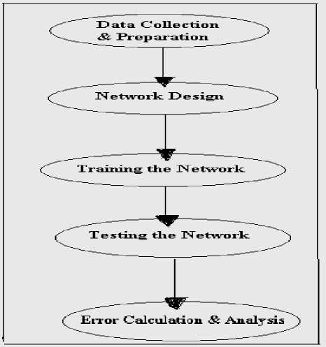
Fig.4. Proposed Methodology

• A.    Data Collection Preparation

The experimental set-up for any machine-learning technique is a two-step process. It includes training and testing of neural network. For each step, specific relevant data set is required. We selected COCOMO dataset (63

projects database by Boehm) for training [2] and the Kemmerer dataset (15 projects database by Kemmerer) [27] for testing.

After making the selection of dataset, the next crucial aspect is data preparation. It is about paying special attention towards how the data is being fed to the network, because the entire performance is very sensitive to the data and its presentation.

Here, this experiment requires three transformations. First, the KDSI is transformed into its corresponding logarithmic value. Second, the actual effort values are translated into logarithmic values. Third, the mode of project is represented with combination of 3-digit Boolean value where Embedded= 1 0 0, Semi-detached= 0 1 0, Organic= 0 0 1 . The basic reason behind these conversions is that all input variables should vary over a roughly similar range between the minimum and maximum values.

Sample Input-output Vector demonstrating transformations shown in Table 3.

The training data set consists of 63 samples. "COCOMO_Inputs" is a 20 x 63 matrix of values. "COCOMO_Targets" is an 1 x 63 matrix. All of the 63 COCOMO projects were used as the training set, and Kemmerer data set of 15 projects were used as the testing set with "KER_Inputs" is a 20 x 15 matrix of values. "KER_Targets" is an 1 x 15 matrix..

Table 3. Sample Input-output Vector demonstrating transformations

Project #1 Attributes as Network I/O	Attributes	Original Data from COCOMO (sample project 1)	Transformed data to feed network (sample fact 1)	Transformation
Input 1	Total KDSI	113	2.03307*^	#1
Input 2	AAF	1	1
Input 3	RELY	0.88	0.88
Input 4	DATA	1.16	1.16
Input 5	CPLX	0.7	0.7
Input 6	TIME	1	1
Input 7	STOR	1.06	1.06
Input 8	VIRT	1.15	1.15
Input 9	TURN	1.07	1.07
Input 10	ACAP	1.19	1.19
Input 11	AEXP	1.13	1.13
Input 12	PCAP	1.17	1.17
Input 13	VEXP	1.1	1.1
Input 14	LEXP	1	1
Input 15	MODP	1.24	1.24
Input 16	TOOL	1.1	1.1	Transformation
Input 17	SCED	1.04	1.04	#3
Input 18	MODE	Embedded	1
Input 19			0	Transformation
Input 20			0	#2
Output 1	Actual EFFORT	2040	3.30963

• B.    Proposed Model

Designing the neural network is an iterative process.

Prior to the training, no configuration can be said the best arrangement. Various network configurations iteratively trained in the ranges of Number of Hidden Neurons: 1-10;

12-20; 20-30 and Number of Hidden Layers: 1-2 ; 1-2 ; 1-2 to search for the best-performing configurations. Our worthy efforts lead us to following six top configurations of network.

The proposed model SG [N1/N2] is a feed forward back-propagation multilayer neural network, comprised of one input layer, one output layer and two hidden layers shown in fig. 5.

The size of input layer is 20 input neurons where each neuron represents one particular software attribute on which effort depends. Output layer produces effort estimated as a single output. The size of hidden layers varies in different configurations. Other parameters are same in all six configurations like transfer function, training function etc.

Proposed model with five Configurations:

Configuration I. SG1 [5/8] with N1=5; N2=8;

Configuration II. SG2 [8/9] with N1=8; N2=9;

Configuration III. SG3 [11/10] with N1=11; N2=10;

Configuration IV. SG4 [16/19] with N1=16; N2=19;

Configuration V. SG5 [18/15] with N1=18; N2=15; Configuration VI. SG6 [24/25] with N1=24; N2=25;

where N1 = number of neurons in 1st Hidden Layer and N2 = number of neurons in 2nd Hidden Layer

The sigmoid function is selected as transfer function at hidden layers. The sigmoid or S-shape that ranges asymptotically between zero and one. The reason for choosing the sigmoid is that the function must be continuously differentiable and should be asymptotic for infinitely large positive and negative values of the independent variables [11]. At output layer pure linear function is selected as transfer function. While training, Mean Squared Error is Performance function. For training back-propagation algorithm based on Delta rule is employed via Levenberg-Marquardt back-propagation function.

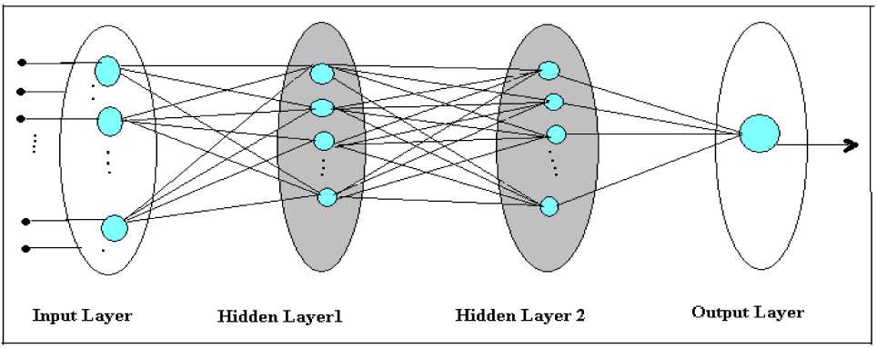
Fig.5. Overall Architecture of Proposed Model

• C.    Performance Evaluation Criteria

The performance of proposed model can be evaluated as the degree to which the model’s estimated effort (Effort Estimated ) matches the actual effort (Effort Actual ). If the model would be perfect, then for every project Effort Estimated = Effort Actual .

Boehm [2] introduced percentage error test with

Percentage Error = Effort- Estimated - Effort Actual Effort Actual

Estimation may vary as over-estimation or as under-estimation; Overestimation results into either less production (Parkinson’s law: “Work expands to fill the time available for its completion”) or add so-called “gold plating” [2]. Underestimation may lead the project understaffed and new staff would be appointed as the deadlines approaches. This results in a heavy loss (Brooks’s law: “Adding man-power to a late software project makes it later” ) [32]. Conte et al. [33] suggested a magnitude of relative error, or MRE Test taking in consideration both under-estimation and over-estimation.

MRE =

Effort Estimated - Effort Actual

EffortActual

ESTIMATION   ACCURACY   EVALUATION

CRITERIA # 1

The Magnitude of Relative Error (MRE) and the Mean Magnitude of Relative Error (MMRE) [34], [35] are used to evaluate the accuracy of the cost estimation models. They are defined as:

MRE =

y - У yi

where y i is the actual value and ỹ i is the estimate.

E MREi MMRE = -i=1----- n where n is the number of estimates; and is the Magnitude of Relative Error (MRE) of the ith estimate. The perfect value of the MRE, MMRE test would be zero.

ESTIMATION   ACCURACY   EVALUATION

CRITERIA # 2

The Standard Deviation of Magnitude of Relative Error (SDMRE) is adopted as another evaluation criteria defined as: the standard deviation of MRE for all n estimations made. The perfect value of the SDMRE test would be zero.

ESTIMATION   ACCURACY   EVALUATION

CRITERIA # 3

The Correlation co-efficient, Squared R, is next measurement criteria. This entity reflects the degree to which the model’s estimation correlate with the actual results. Albrecht’s test by performing the linear Regression with actual Effort as the dependent variable and the estimated Effort as the independent variable; is carried out for all proposed models. The perfect value of the R2 test would be one.

• V. Training and Testing the Proposed Model

The proposed model SG [N1/N2] is a feed forward back-propagation multilayer neural network, comprised of one input layer, one output layer and two hidden layers shown in fig.6. The size of input layer is 20 input neurons where each neuron represents one particular software attribute on which effort depends. Output layer produces effort estimated as a single output. The size of hidden layers varies in different configurations. Other parameters are same in all six configurations like transfer function, training function etc.

Proposed model with five Configurations:

Configuration I. SG1 [5/8] with N1=5; N2=8;

Configuration II. SG2 [8/9] with N1=8; N2=9;

Configuration III. SG3 [11/10] with N1=11; N2=10;

Configuration IV. SG4 [16/19] with N1=16; N2=19;

Configuration V. SG5 [18/15] with N1=18; N2=15;

Configuration VI. SG6 [24/25] with N1=24; N2=25;

where N1 = number of neurons in 1st Hidden Layer and N2 = number of neurons in 2nd Hidden Layer

PROPOSED MODEL (SG)

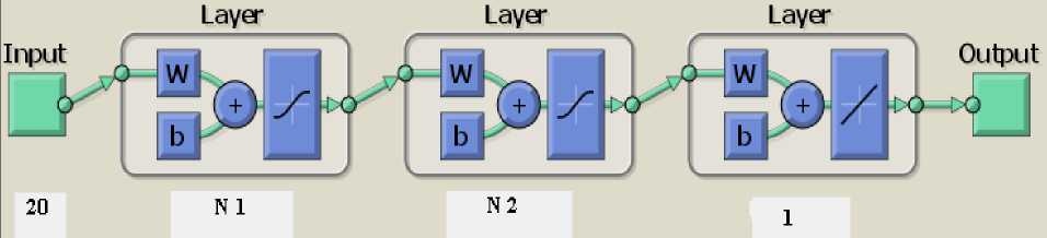
Fig.6. Proposed Model SG[N1/ N2]

• A.    Training of Model SG1 through SG6 with 63 Project COCOMO Dataset

0.47712

1

1.15

0.94

1.65

1.3

1.56

1.15

1

0.86

1

0.7

1.1

1.07

1.1

1.24

1.23

0

1

0

1.86332

0.59106

1

1.4

0.94

1.3

1.3

1.06

1.15

0.87

0.86

1.13

0.86

1.21

1.14

0.91

1

1.23

1

0

0

1.78533

0.78533

0.6

1.4

1

1.3

1.3

1.56

1

0.87

0.86

1

0.86

1

1

1

1

1

1

0

0

1.60206

0.5563

0.53

1.4

1

1.3

1.3

1.56

1

0.87

0.86

0.82

0.86

1

1

1

1

1

1

0

0

0.95424

2.50515

1

1.15

1.16

1.15

1.3

1.21

1

1.07

0.86

1

1

1

1

1.24

1.1

1.08

1

0

0

4.0569

3.06069

0.84

1.15

1.08

1

1.11

1.21

0.87

0.94

0.71

0.91

1

1

1

0.91

0.91

1

1

0

0

3.81954

2.47567

0.96

1.4

1.08

1.3

1.11

1.21

1.15

1.07

0.71

0.82

1.08

1.1

1.07

1.24

1

1.08

0

1

0

3.80618

2.4014

1

1

1.16

1.15

1.06

1.14

0.87

0.87

0.86

1

1

1

1

0.91

0.91

1

1

0

0

3.39005

2.07188

0.92

1.15

1

1

1.27

1.06

1

1

0.86

0.82

0.86

0.9

1

0.91

1

1.23

1

0

0

2.85973

1.88649

0.98

1.15

1

1

1.08

1.06

1

1

0.86

0.82

0.86

0.9

1

1

1

1.23

1

0

0

2.73158

1.95424

1

0.88

1

0.85

1.06

1.06

1

0.87

1

1.29

1

1.1

0.95

0.82

0.83

1

0

1

0

2.65609

1.57978

1

1.15

1.16

1.3

1.15

1.06

1

0.87

0.86

1

0.86

1.1

1

0.82

0.91

1.08

1

0

0

2.7185

1.68124

1

0.94

1

0.85

1.07

1.06

1.15

1.07

0.86

1

0.86

1.1

1

0.91

1.1

1.08

1

0

0

2.58771

0.97312

1

1.15

0.94

1.15

1.35

1.21

1

0.87

1

1

1

1

1

0.82

1.1

1.08

1

0

0

1.94448

1.11394

1

1.15

1.08

1.3

1.11

1.21

1.15

1.07

0.86

1

0.86

1.1

1.07

1.1

1.1

1

0

0

1

1.99122

0.33041

1

0.88

1

1

1

1

1

1

1.1

1.29

0.86

1

1

0.91

0.91

1.23

0

1

0

0.86332

0.29666

1

0.88

1

1

1

1

1

1

1.1

1.29

0.86

1

1

0.91

0.91

1.23

0

1

0

0.77085

1.79239

0.81

1.4

1.08

1

1.48

1.56

1.15

1.07

0.86

0.82

0.86

1.1

1.07

1

1

1

1

0

0

3.02653

2.59106

0.67

0.88

1.08

0.85

1

1

1

1

0.71

0.82

1

1

1

1.1

1.1

1

0

1

0

2.84633

1.62324

0.96

1.4

1.08

1.3

1.48

1.56

1.15

0.94

0.86

0.82

0.86

0.9

1

0.91

0.91

1

1

0

0

2.78175

1.36172

0.96

1.15

1.08

1

1.06

1

1

0.87

1

1

1

1

1

0.91

1.1

1.23

1

0

0

2.36172

1.11394

1

0.75

0.94

1.3

1.06

1.21

1.15

1

1

0.91

1

1.1

1

1.24

1.24

1

1

0

0

1.91381

1.17609

0.81

0.88

1.08

0.85

1

1

0.87

0.87

1.19

1

1.17

0.9

0.95

1

0.91

1.04

0

1

0

1.74036

1.77815

0.56

0.88

0.94

0.7

1

1.06

1

1

0.86

0.82

0.86

1

1

1

1

1

0

0

1

1.67209

1.17609

1

1

1

1.15

1

1

0.87

0.87

0.71

0.91

1

0.9

0.95

0.82

0.91

1

0

0

1

1.07918

0.47712

0.83

1

0.94

1.3

1

1

1

0.87

0.86

0.82

1.17

1

1

1.1

1

1

0

0

1

0.90309

0.72427

1

0.88

0.94

1

1

1

0.87

0.87

1

0.82

0.7

0.9

0.95

0.91

0.91

1

0

0

1

0.77815

1.65801

0.43

0.88

1.04

1.07

1

1.06

0.87

1.07

0.86

1

0.93

0.9

0.95

0.95

0.95

1.04

0

0

1

1.65321

1.45636

0.98

1

1.04

1.07

1

1.21

0.87

1.07

0.86

1

1

0.9

0.95

1

1

1.04

0

0

1

1.91907

1.48572

0.98

0.88

1.04

1.07

1.06

1.21

0.87

1.07

1

1

1

0.9

0.95

1.1

1

1.04

0

0

1

1.93951

1.54406

0.91

0.88

1.04

1.07

1

1.06

0.87

1.07

1

1

1

0.9

0.95

1

0.95

1.04

0

0

1

2.0253

1.86332

0.78

0.88

1.04

1.07

1

1.06

0.87

1.07

1

1

0.86

0.9

0.95

1

1

1.04

0

0

1

2.10037

1.36172

1

0.75

0.94

1.3

1

1

0.87

0.87

0.71

0.82

0.7

1.1

1.07

1.1

1

1.04

0

0

1

1.5563

2.66651

0.67

0.88

0.94

0.85

1

1

0.87

1

1.19

0.91

1.17

0.9

0.95

1.1

1

1.04

0

1

0

3.10448

1.95904

1

1

1

0.85

1

1

1

0.87

0.71

1

0.7

1.1

1

0.82

0.91

1

0

1

0

2.19312

1.38021

1

1.15

1

1

1.3

1.21

1

0.87

0.86

1

0.86

1.1

1

1

1

1

1

0

0

2.24551

1

1

0.88

1

1

1

1

1

1.15

1.19

1

1.42

1

0.95

1.24

1.1

1.04

0

0

1

2.08636

0.91381

1

0.88

0.94

0.85

1

1.06

1.15

1

1

1

1

1.1

1.07

1.24

1.1

1

0

0

1

1.61278

0.72427

1

0.88

0.94

1.15

1.11

1.21

1.3

1

0.71

1

0.7

1.1

1.07

1

1.1

1.08

0

1

0

1.14612

0.64345

1

1

0.94

1

1

1.06

1.15

0.87

1

0.82

1

1

0.95

0.91

1.1

1

0

0

1

1.30103

0.79934

1

0.88

0.94

0.7

1

1

0.87

0.87

0.86

0.82

1.17

0.9

0.95

1.1

1

1

0

0

1

1.25527

1.43136

1

1.15

0.94

1.3

1.3

1.21

1

1

0.86

0.91

1

1.1

1.07

1.1

1.1

1.08

1

0

0

2.98136

1.23044

0.87

1

0.94

1.15

1.11

1.21

1.3

1

1

1

1

1.1

1.07

1.1

1.1

1.23

1

0

0

2.37474

1.39794

1

1.4

0.94

1.3

1.66

1.21

1

1

0.71

0.82

0.7

0.9

0.93

0.91

1

1

1

0

0

2.11394

1.36172

0.9

1

0.94

1.15

1.06

1.06

1

0.87

1

1

1

1

1

0.91

1

1

0

0

1

1.84509

0.82607

1

1.15

0.94

1.3

1.11

1.06

1

1

0.86

1.13

0.86

1.1

1.07

1.1

1.1

1.08

0

0

1

1.75587

1.44715

1

1

0.94

1.15

1

1

0.87

0.87

0.86

1

0.86

0.9

1

0.82

1

1

0

0

1

1.69897

0.95904

1

0.88

0.94

1.3

1.11

1.21

1.15

1

0.78

0.82

0.7

1.21

1.14

0.91

1.24

1

0

1

0

1.57978

1

1

1

0.94

1.15

1

1

1

0.87

0.71

0.82

0.86

1

1

0.82

1

1

1

0

0

1.17609

Table 4. 63 Project COCOMO Dataset for Training

Total KDSI	AAF	RELY	DATA	CPLX	TIME	STOR	VIRT	TURN	ACAP	AEXP	PCAP	VEXP	LEXP	MODP	TOOL	SCED	MODE1	MODE2	MODE3	Effort
2.03307	1	0.88	1.16	0.7	1	1.06	1.15	1.07	1.19	1.13	1.17	1.1	1	1.24	1.1	1.04	1	0	0	3.30963
2.46686	0.85	0.88	1.16	0.85	1	1.06	1	1.07	1	0.91	1	0.9	0.95	1.1	1	1	1	0	0	3.20412
2.12057	1	1	1.16	0.85	1	1	0.87	0.94	0.86	0.82	0.86	0.9	0.95	0.91	0.91	1	0	1	0	2.3856
1.77815	0.76	0.75	1.16	0.7	1	1	0.87	1	1.19	0.91	1.42	1	0.95	1.24	1	1.04	0	0	1	2.38021
1.20412	1	0.88	0.94	1	1	1	0.87	1	1	1	0.86	0.9	0.95	1.24	1	1	0	0	1	1.51851
0.60206	1	0.75	1	0.85	1	1.21	1	1	1.46	1	1.42	0.9	0.95	1.24	1.1	1	0	0	1	1.63346
0.83884	1	0.75	1	1	1	1	0.87	0.87	1	1	1	0.9	0.95	0.91	0.91	1	0	0	1	0.90309
1.34242	1	1.15	0.94	1.3	1.66	1.56	1.3	1	0.71	0.91	1	1.21	1.14	1.1	1.1	1.08	1	0	0	3.0314
1.47712	1	1.15	0.94	1.3	1.3	1.21	1.15	1	0.86	1	0.86	1.1	1.07	0.91	1	1	1	0	0	2.62634
1.46239	0.63	1.4	0.94	1.3	1.11	1.56	1	1.07	0.86	0.82	0.86	0.9	1	1	1	1	1	0	0	2.5065
1.50515	0.63	1.4	0.94	1.3	1.11	1.56	1	1.07	0.86	0.82	0.86	0.9	1	1	1	1	1	0	0	2.33845
1.5682	1	1.15	0.94	1.3	1.11	1.06	1	1	0.86	0.82	0.86	1	0.95	0.91	1	1.08	1	0	0	2.30319
1.39794	0.96	1.15	0.94	1.3	1.11	1.06	1.15	1	0.71	1	0.7	1.1	1	0.82	1	1	1	0	0	1.89762

• B.    Testing of Model SG1 through SG6 with 15 Project KEMERER Dataset

Table 5. Kemerer Dataset

Total KDSI	AAF	RELY	DATA	CPLX	TIME	STOR	VIRT	TURN	ACAP	AEXP	PCAP	VEXP	LEXP	MODP	TOOL	SCED	MODE1	MODE2	MODE3	Effort
2.40414	1	1.15	1.08	1.15	1	1.06	0.87	1	0.86	1.13	0.86	1	1	0.82	0.91	1.02	0	1	0	2.45788
1.60745	1	1	1	1	1	1	0.87	1	1	1.07	0.86	1	1	1	1	1	0	1	0	1.91645
2.65321	1	1	1.16	1	1.3	1.21	0.87	1	0.86	1.13	1	1	1.03	0.91	1	1	1	0	0	3.04426
2.33122	1	1	1.08	0.92	1	1	0.87	0.93	0.8	0.89	0.85	0.97	0.95	1	1	1.02	0	1	0	1.93019
2.65311	1	1	0.94	1	1	1	0.93	0.87	0.78	1.13	0.93	1.1	1.03	1	0.91	1.07	0	0	1	2.52673
1.69897	1	1	1.16	1	1.11	1.06	1	0.87	0.86	1.13	0.86	0.95	0.97	0.91	1	1.23	1	0	0	1.92428
1.63346	1	1	1.16	1	1.11	1.06	1	0.87	0.86	1.13	0.7	0.95	1.07	0.91	1	1.23	1	0	0	1.36549
2.22271	1	1.15	1.16	1	1	1	1	0.93	1	0.95	1	0.95	0.97	1	1	1.16	0	1	0	2.11494
2.46089	1	1	1.16	1.15	1.11	1.06	0.87	0.87	1	1.13	1.06	1.1	1	1	1	1.08	1	0	0	2.06446
1.59106	1	1	1.16	1	1.11	1	0.93	1.03	0.71	1	0.7	1.1	1.14	1.05	1	1.23	0	1	0	1.85733
2.40517	1	1.16	1	1	1	1	1	1	0.86	1.13	0.86	1	1	0.86	1	1.23	0	1	0	2.4128
2.10924	1	1	1.16	1	1	1	0.87	0.87	0.86	1.07	0.86	1	1.03	1.1	0.95	1.08	0	1	0	2.36305
2.2079	1	1	1.16	1	1.06	1	0.87	0.87	1.19	1	0.78	1.21	0.97	1.1	1	1.08	0	1	0	2.19589
2.21695	1	1	1.16	1	1	1	0.87	0.87	0.86	1.21	0.93	1.1	1.1	0.95	0.91	1.04	0	0	1	2.39252
1.77959	1	1	1	1	1	1	1	0.87	0.71	0.91	0.86	1.1	1.03	0.91	0.91	1	0	1	0	1.84447

Fig.7. Sample Training of Model SG[N1/ N2]

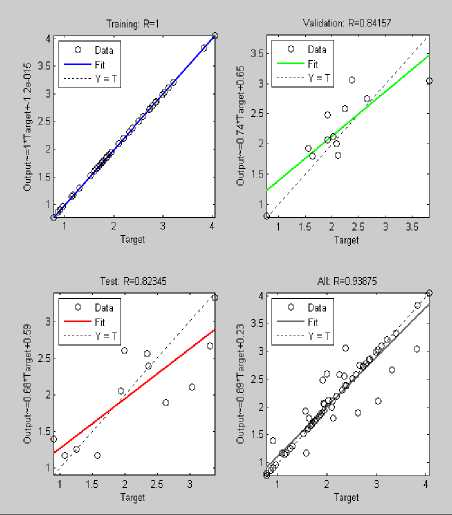
Fig.8. Sample Testing of Model SG[N1/ N2]

• VI.    Experiment Results and Analysis of Performance

The analysis on the performance of the proposed model with all six configuration is made taking in consideration evaluation criteria MRE, MMRE SDMRE and correlation coefficient, squared R. Selection of these aforementioned criterion is purely inspired from the work done by great Kemerer [27], that the analysis of the performance of various software cost estimation models using the same Kermerer 15 project data set and these three performance criteria.

Kermerer data for 15 projects is being used in the testing of our proposed model. The closer MRE/MMRE/SDMRE value is to zero, the greater is the accuracy of the model. The closer R-squared measure is to one, the better is the correlation between the estimates of each model and the actual project results.

• A.    Performance of the proposed model

Our experimentation begins with the training of proposed models shown fig. 9, using entire 63 project COCOMO data set which is followed by testing using 15 project Kemmerer data set.

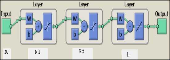
Fig.9. Proposed Model SG[N1/ N2]

Proposed Model SG[N1/ N2] with six top Configurations:

• I.    SG1 [5/8] with N1=5; N2=8;

• II.    SG2 [8/9] with N1=8; N2=9;

• III.    SG3 [11/10] with N1=11; N2=10;

• IV.    SG4 [16/19] with N1=16; N2=19;

• V.    SG5 [18/15] with N1=18; N2=15;

• VI.    SG6 [24/25] with N1=24; N2=25;

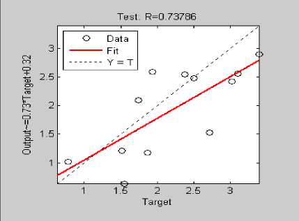
Fig.10. Correlation Coefficient SG 1 [5 / 8]

Table 7. Performance statistics for Configuration II: SG2: N1=8; N2=9;

Configuration III : SG3: N1=11; N2=10;
Project No.	Actual Effort (in MM)	Estimated Effort (in MM)	Error %
1	287.00	1412.07	3.92
2	82.50	222.89	1.70
3	1107.31	4615.97	3.16
4	86.90	709.90	7.33
5	336.30	3545.32	9.54
6	84.00	391.53	3.66
7	23.20	120.71	4.20
8	130.30	674.71	4.17
9	116.00	3485.23	29.04
10	72.00	80.184	0.11
11	258.70	654.12	1.52
12	230.70	287.37	0.24
13	157.00	179.52	0.14
14	246.90	351.78	0.42
15	69.90	67.17	-0.03
MMRE 461.16
Standard Deviation SDMRE 731.40

Table 6. Performance statistics for Configuration I: SG1: N1=5; N2=8

Configuration I : SG1: N1=5; N2=8;
Project No.	Actual Effort (in MM)	Estimated Effort (in MM)	Error %
1	287.00	400.32	0.39
2	82.50	81.39	-0.013
3	1107.31	682.66	-0.38
4	86.90	246.18	1.89
5	336.30	145.50	-0.56
6	84.00	449.07	4.34
7	23.20	504.79	20.75
8	130.30	471.7	2.62
9	116.00	746.61	5.43
10	72.00	218.75	2.038
11	258.70	606.17	1.34
12	230.70	220.21	-0.04
13	157.00	90.48	-0.42
14	246.90	176.46	-0.28
15	69.90	36.84	-0.47
MMRE 244.24
Standard Deviation SDMRE 539.42

Performance statistics for Configuration I: SG1: N1=5; N2=8; is shown in Table VI with 0.737 correlation coefficient displayed in fig.10. Minimum MRE is 0.013 and maximum MRE is 20.75.

Performance statistics for Configuration II: SG2: N1=8; N2=9; is shown in Table VII with 0.786 correlation coefficient fig.11. Minimum MRE is 0.05 and maximum MRE is 34.02.

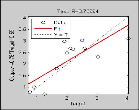
Fig.11. Correlation Coefficient SG 2 [8 / 9]

Performance statistics for Configuration III: SG3: N1=11; N2=10; is shown in Table VIII with 0.8516 correlation coefficient displayed fig.12. Minimum MRE is 0.03 and maximum MRE is 29.04. The estimation is fairly good correlated with actual effort.

Table 8. Performance statistics for Configuration III: SG3: N1=11;

N2=10;

Configuration II : SG2: N1=8; N2=9;
Project No.	Actual Effort (in MM)	Estimated Effort (in MM)	Error %
1	287.00	531.04	0.85
2	82.50	322.16	2.90
3	1107.31	907.79	-0.18
4	86.90	1125.75	12.22
5	336.30	530.77	0.57
6	84.00	181.76	1.16
7	23.20	167.18	6.20
8	130.30	169.76	0.30
9	116.00	4062.85	34.024
10	72.00	280.68	2.89
11	258.70	144.30	-0.44
12	230.70	736.35	2.19
13	157.00	148.40	-0.05
14	246.90	1455.58	4.89
15	69.90	605.96	7.66
MMRE 501.52
Standard Deviation SDMRE 876.43

Performance statistics for Configuration IV: SG4: N1=16; N2=19; is shown in Table IX with 0.929 correlation coefficient displayed fig.12. Minimum MRE is 0.70 and maximum MRE is 20.20. The estimation is strongly correlated with actual effort nearly to the perfect score (~1).

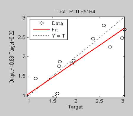
Fig.12. Correlation Coefficient SG 3 [11 / 10]

Table 9. Performance statistics for Configuration IV: SG4: N1=16;

N2=19;

Configuration IV : SG4: N1=16; N2=19;
Project No.	Actual Effort (in MM)	Estimated Effort (in MM)	Error %
1	287.00	81.91	-0.71
2	82.50	10.38	-0.87
3	1107.31	6522.10	4.89
4	86.90	520.21	5.10
5	336.30	6.10	-0.98
6	84.00	689.01	7.20
7	23.20	199.29	7.59
8	130.30	494.36	2.79
9	116.00	2460.13	20.20
10	72.00	380.59	4.28
11	258.70	98.49	-0.61
12	230.70	394.09	0.70
13	157.00	1245.69	6.93
14	246.90	48.49	-0.80
15	69.90	418.91	4.99
MMRE 404.82
Standard Deviation SDMRE 550.98

Performance statistics for Configuration V: SG5: N1=18; N2=15; is shown in Table X with 0.904 correlation coefficient displayed in fig. 14. Minimum MRE is 0.03 and maximum MRE is 10.33. The estimation is strongly correlated with actual effort nearly to the perfect score (~1). The overall deviation is very low.

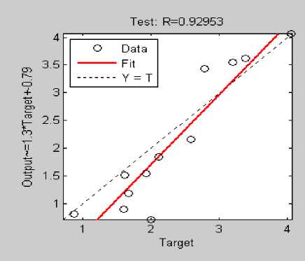
Fig.13. Correlation Coefficient SG 4 [ 16 / 19 ]

Table 10. Performance statistics for Configuration V: SG5: N1=18;

N2=15;

Configuration V : SG5: N1=18; N2=15;
Project No.	Actual Effort (in MM)	Estimated Effort (in MM)	Error %
1	287.00	651.20	1.26
2	82.50	104.06	0.26
3	1107.31	3816.78	2.44
4	86.90	165.35	0.94
5	336.30	141.49	-0.57
6	84.00	79.44	-0.05
7	23.20	97.43	3.19
8	130.30	723.60	4.55
9	116.00	1047.97	8.03
10	72.00	815.94	10.33
11	258.70	572.57	1.21
12	230.70	164.05	-0.28
13	157.00	162.67	0.03
14	246.90	324.18	0.31
15	69.90	253.49	2.62
MMRE 228.70
Standard Deviation SDMRE 317.65

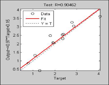
Fig.14. Correlation Coefficient SG 5 [18 / 15]

Performance statistics for Configuration VI : SG6: N1=24; N2=25; is shown in Table 11 with 0.831 correlation coefficient displayed in fig. 15. Minimum MRE is 0.15 and maximum MRE is 15.75. The estimation is nicely correlated with actual effort.

Table 11. Performance statistics for Configuration VI: SG6: N1=24;

N2=25;

Configuration VI : SG6: N1=24; N2=25;
Project No.	Actual Effort (in MM)	Estimated Effort (in MM)	Error %
1	287.00	85.54	-0.70
2	82.50	6.86	-0.91
3	1107.31	3537.47	2.19
4	86.90	98.19	0.15
5	336.30	14.62	-0.95
6	84.00	609.75	6.25
7	23.20	388.72	15.75
8	130.30	247.99	0.90
9	116.00	1024.60	7.83
10	72.00	292.15	3.05
11	258.70	73.58	-0.71
12	230.70	131.65	-0.42
13	157.00	763.08	3.86
14	246.90	48.69	-0.80
15	69.90	209.64	1.99
MMRE 249.95
Standard Deviation SDMRE  457.11

Overall performance as in Table 12 of all configurations suggests that SG5 is the best performer among all six top configurations. SG5 with 18 neurons at hidden layer 1 and 15 neurons at hidden layer 2 gives the best results with minimum MMRE and Standard deviation. The correlation coefficient is quite high. Fig. 16 shows the bar plot for SG1 through SG6.

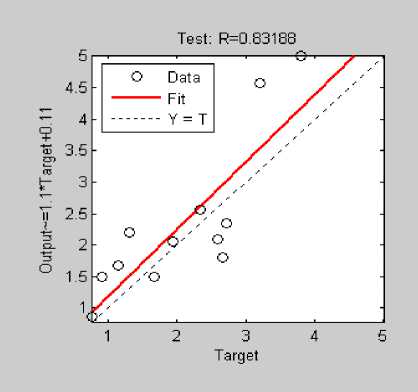
Fig.15. Correlation Coefficient SG 6[24 / 25]

Table 12. Performance of Proposed Model (SG)

Performance of Proposed Model (SG)
Configuration	Approach	MMRE %	Standard Deviation SDMRE %	Correlation (Estimated Vs. Actual)
I	SG1 [5/8]	244.24	539.42	0.737
II	SG2 [8/9]	501.52	876.43	0.786
III	SG3 [11,10]	461.16	731.40	0.851
IV	SG4 [16/19]	404.82	550.98	0.929
V	SG5 [18/15]	228.70	317.65	0.904
VI	SG6 [24/25]	249.95	457.11	0.831

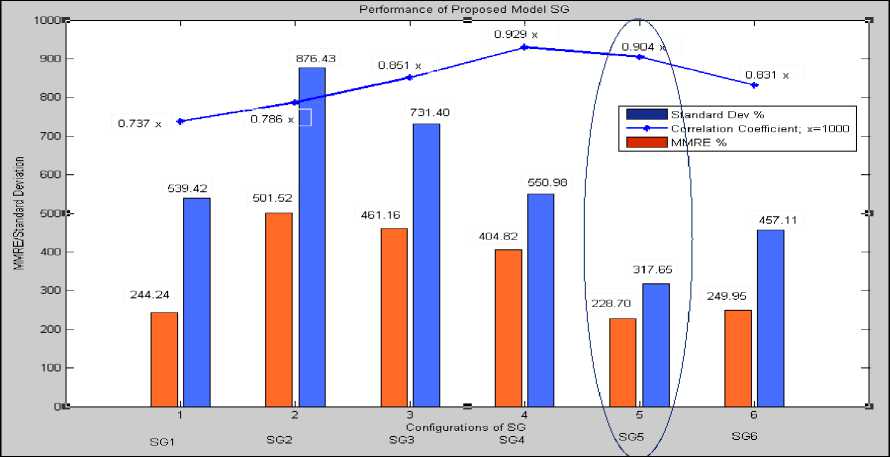
Fig.16. The bar plot for SG1 through SG6.

• B.    Comparison of proposed model with traditional models

At this step of experimentation, it is possible to compare the estimating capability of the machine learning based proposed model with traditional models referring the results obtained by Kemmerer [27]. Various models are SLIM, ESTIMACS,

Function Points, and COCOMO. These results shown in Table 13 serve as an indication about the machine generated models’ capability to generalize across multiple development domains that seems critical for any model while considering the success of the project.

Table 13 . Comparison of proposed model with traditional models

Model	MMRE %	Standard Deviation SDMRE %	Correlation (Estimated Vs. Actual)
SG1 [5/8]	244.24	539.42	0.737
SG2 [8/9]	501.52	876.43	0.786
SG3 [11,10]	461.16	731.40	0.851
SG4 [16/19]	404.82	550.98	0.929
SG5 [18/15]	228.70	317.65	0.904
SG6 [24/25]	249.95	457.11	0.831
ESTIMACS [27]	85.48	70.36	0.134
Function Point [27]	102.74	112.11	0.553
SLIM [27]	771.87	661.33	0.878
Intermediate-COCO MO [27]	583.82	862.79	0.599

Table 14. Comparison of proposed model with traditional models

Model	MMRE %
SG1 [5/8]	244.24
SG2 [8/9]	501.52
SG3 [11,10]	461.16
SG4 [16/19]	404.82
SG5 [18/15]	228.70
SG6 [24/25]	249.95
MayaZaki and Mori (1985)	165.60
Kemerer (1987)	583.82
Chandrasekaran and Kumar (2012)	8.4
Weighted Average	284.61

The best network is SG5 [18/15] with an accuracy greater than that of either SLIM or Intermediate COCOMO and a correlation factor higher than all of the traditional models. While none of the networks could be considered truly accurate, the results of this experiment indicate that networks are worth strong consideration shown in fig. 17.

Only SLIM has somewhat comparable Correlation coefficient with SG5 as shown in fig. 18, but MMRE and standard deviation are worse.

• C.    Comparison of proposed model with traditional models

The proposed model with configuration SG5 [18/15] shows MMRE at 228.70 % while till date COCOMO accuracy reported is with MMRE at 284.61. It clearly reflects the improvement in COCOMO model while sustaining the desirable features of COCOMO and machine learning aspect of Neural network shown in Table 14.

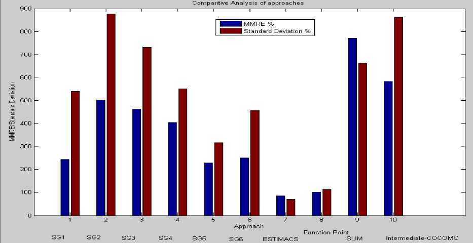
Fig.17. Comparative analysis of Models

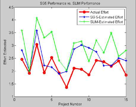
Fig.18. SG5 Performance Vs. SLIM Performance

• VII.    Conclusion

Accurate effort estimation is highly crucial in the software development. Through this presented work, first up major accuracy reports of COCOMO performance are reviewed. Along this, wide range of estimation methods is reviewed. It is found that every method played important role in software development history. Various research reports have been contributed by dignified authors. But no model is adaptive to the latest development methods, resulting into the project failures. In such scenario, Machine learning is the answer to find out the relationship existing among the software project attributes and the effort required for the successful completion of the project. The core objective for this entire work is to apply machine learning technique to improve performance of COCOMO estimation model.

Neural network finds out such relationships during the training phase and then can be exploited to predict the estimate for unseen data. Our traditional estimation techniques are not able to capture and record such patterns as ML techniques do. Hence, ML based models are superior to the traditional models. Neural network as a tool deployed in the research work carried out here. Neural networks are having a strong capability to capture and learn the project data and predict effort with accuracy and a high degree of correlation with the project actual values.

The proposed model shows best performance to generalize on the data and make estimates better than those of other well-known models. Proposed models SG5 trained using COCOMO dataset and tested for KEMERER dataset gives best 0.9 Correlation coefficient with 228.70 MMRE % and 317.65 SDMRE % which is superior to reported accuracy of COCOMO that is 284.61 MMRE %.

This feature of making estimation across domains is critical when applied to the new development domains. Our proposed model performed quite well. An advantage of deploying neural networks is the ease to set up and train them within the range of project personnel. Further, proposed model is self-calibrating sort of tool when fed with data of newly completed projects and retrained. Although, accuracy of the proposed model is not as that of algorithmic models, but it is worthy as per their performance and ability to deal with non-numeric, or symbolic, data. The proposed can be directly applied within an organization at the earliest stages of project to capture the likely magnitude of the project under consideration. The models SG1 through SG6 are fairly accurate and strongly correlated. These results indicate that machine learning shows great usefulness as an exciting new approach to the cost estimation problem.