Machine Learning for Weather Forecasting: XGBoost vs SVM vs Random Forest in Predicting Temperature for Visakhapatnam

In the arena of modern global concerns, climate change, marked by significant and enduring transformations in the patterns of global weather, stands as one of the most intricate and urgent challenges of our era. This potent worldwide phenomenon is precipitously upending the erstwhile predictability of our planet's temperature dynamics, thereby fostering an environment characterized by increased volatility and uncertainty. Among the myriad adverse manifestations of climate change, the disturbances in temperature patterns emerge as particularly significant, posing substantial threats to a multitude of human and environmental systems, and influencing sectors as wide-ranging as agriculture, energy, public health, and numerous others. Consequently, in this unfolding scenario of climatic upheaval, the capability to predict temperature with both accuracy and timeliness has evolved into an indispensable tool. Forecasts pertaining to temperature, particularly those addressing daily maximum and minimum ranges, find themselves central to an extensive gamut of practical applications. For instance, in the realm of agricultural operations, precise temperature forecasts can provide crucial guidance to the formulation of effective planting and harvesting schedules. Similarly, in the energy sector, such predictions can facilitate the delicate balancing act of supply and demand dynamics. Furthermore, in the sphere of public health, accurate temperature forecasts are instrumental in enabling preparedness for temperature-related extreme events such as heatwaves. Additionally, these forecasts serve a critical function in shaping strategies aimed at both mitigating the impacts of climate change and adapting to its inevitable consequences.

Historically, the task of temperature forecasting has been largely reliant on physical models. While these traditional methods have demonstrated considerable effectiveness, they frequently encounter difficulties when confronted with the inherent non-linearity and complexity characteristic of climatic systems. With the emergence and rapid advancement of machine learning (ML) technologies, an innovative pathway has been unveiled to address these complications. ML algorithms, with their inherent capability to learn from vast datasets and capture non-linear relationships, represent a promising complement or alternative to conventional forecasting methodologies.

In recent years, the spotlight of the scientific community has been increasingly focused on several ML techniques due to their robust predictive performance across a myriad of fields. Notable among these techniques are eXtreme Gradient Boosting (XGBoost), Support Vector Machine (SVM), and Random Forest. Despite the potential exhibited by these techniques, there remains a conspicuous absence of a comprehensive, comparative analysis of their performance within the specific context of temperature forecasting. Moreover, the nuanced implications of model selection, particularly in relation to the specific task and performance measures under consideration, warrant a more thorough exploration.

The major research objectives of this study are to evaluate and compare the performance of XGBoost, SVM, and Random Forest methodologies for predicting daily maximum and minimum temperatures. The study leverages a meticulously curated 45-year dataset from Visakhapatnam airport to assess the effectiveness of these ML models. By conducting a comprehensive intercomparison, the aim is to identify the most suitable model for temperature forecasting and shed light on the critical significance of model selection and alignment of performance metrics.

This research addresses the existing gap by providing insights into the strengths and limitations of different ML models for temperature forecasting. By comparing their performance, the study aims to determine the most effective approach in terms of accuracy and reliability. Furthermore, the research aims to highlight the importance of judicious model selection and the alignment of performance metrics based on the specific requirements of the task at hand.

By achieving these objectives, this research seeks to contribute to the advancement of temperature forecasting techniques and provide valuable guidance for researchers and practitioners in selecting the most appropriate ML model. The ultimate goal is to enhance the accuracy and reliability of temperature predictions, enabling informed decisionmaking and effective climate change mitigation and adaptation strategies.

2.    Literature Review

Temperature prediction plays a crucial role in various domains, and machine learning has emerged as a powerful tool for achieving accurate predictions. A review of relevant literature reveals the potential of machine learning methods such as Random Forests, Support Vector Machines (SVM), and XGBoost in temperature prediction. Random Forests, introduced by Breiman (2001), construct multiple decision trees during training and provide the mode of classes (classification) or mean prediction (regression) of individual trees [1]. This algorithm is renowned for its ability to handle large datasets, avoid overfitting, and robustness to noise and outliers. The study by Caruana and Niculescu-Mizil (2006) comparing Random Forests with other machine learning algorithms provides evidence of its robustness and accuracy [2]. This is relevant to our research objectives as it establishes Random Forests as a potential method for accurate temperature prediction. XGBoost, introduced by Chen and Guestrin (2016), is a scalable machine learning system for tree boosting [3]. It has been praised for its speed and performance, offering a robust framework.

SVMs, presented by Cortes and Vapnik (1995), construct hyperplanes in multidimensional space for classification and regression tasks [4]. They have demonstrated effectiveness in various applications, including temperature prediction. The work of Kavzoglu and Colkesen (2009) showcases the application of SVMs in environmental studies, achieving satisfactory results [5]. Additionally, literature on machine learning methodology offers valuable insights into understanding these algorithms. Book such as 'Fundamentals of machine learning for predictive data analytics' by Kelleher et al. [6] provide comprehensive overviews, enhancing our understanding of the methodologies employed in temperature prediction. In the context of temperature prediction, the study by Liaw and Wiener (2002) [7] demonstrates the potential of Random Forests as a suitable machine learning approach for accurate temperature prediction. It highlights the algorithm's ability to handle both classification and regression problems, its effectiveness in handling large datasets, and its robustness to noise and outliers.

The study by Sani et al. (2021) demonstrates the superior performance of XGBoost over traditional machine learning algorithms in temperature prediction [8]. The relevance of XGBoost to our research objectives lies in its potential as an effective method for accurate temperature prediction.

Comparative studies have been conducted to evaluate the performance of these algorithms. Debnath et al. (2019) compared SVM, Artificial Neural Network (ANN), and Random Forest for temperature prediction and found accurate results with all methods [9]. Faisal et al. (2018) surveyed different machine learning approaches for weather forecasting and emphasized the impact of algorithm choice on prediction performance [10]. These studies provide valuable insights into the comparative performance of different algorithms and their relevance to our research objectives.

Zhang and Qi (2005) explored neural network forecasting for seasonal and trend time series, providing insights into the application of neural networks in temperature prediction [11]. This study is relevant as it highlights an alternative method for temperature forecasting. The work of Laio et al. (2001) on vegetation water stress in water-controlled ecosystems contributes to understanding the role of plants in hydrologic processes and their response to water stress [12]. While not directly focused on temperature prediction, it offers valuable insights into the broader context of environmental factors influencing temperature dynamics. Witten and Frank (2005) provide a comprehensive resource on data mining and machine learning techniques, enhancing our understanding of the methodologies employed in temperature prediction [13]. This book serves as a valuable reference for exploring practical applications of machine learning in the field. Biau and Scornet (2016) conducted a guided tour of Random Forests, offering a detailed understanding of the algorithm's characteristics and performance [14]. This study contributes to our evaluation of Random Forests as a potential method for temperature prediction.

"The Nature of Statistical Learning Theory" [15] by Vapnik (2013) holds significance as it offers valuable insights into the fundamental principles and theoretical underpinnings of machine learning. It provides a deeper understanding of the mathematical framework that supports various machine learning algorithms, including those used for temperature prediction. Hastie, Tibshirani, and Friedman (2009) authored "The elements of statistical learning: data mining, inference, and prediction," which provides comprehensive insights into statistical learning methodologies, including machine learning techniques [16]. This resource enhances our understanding of the underlying principles behind the algorithms considered in temperature prediction. Burges (1998) presented a tutorial on support vector machines (SVM) for pattern recognition, which covers the theoretical foundations and practical aspects of SVMs [17]. This study offers valuable insights into the application of SVMs in temperature prediction. Friedman (2002) described stochastic gradient boosting, a powerful technique that forms the basis for XGBoost, thereby reinforcing the foundation of the XGBoost algorithm [18]. This study contributes to our understanding of the underlying principles of XGBoost and its potential for temperature prediction.

In conclusion, the reviewed literature demonstrates the potential of Random Forests, SVM, and XGBoost as machine learning algorithms for accurate temperature prediction. The studies evaluating their performance, the relevance to our research objectives, and their comparative analysis contribute to our understanding of these methods. The literature also provides insights into the methodology of machine learning, aiding our comprehension of the underlying principles.

3.    Data Description

The primary dataset employed in this study consists of daily temperature records amassed over a substantial period of 45 years (from January1969 to January 2015), from the meteorological station located at Visakhapatnam airport. The dataset is comprehensive, featuring robust and reliable daily observations of both maximum and minimum temperatures. The site was selected for its long-standing record of consistent and high-quality data collection, making it an ideal case study for the machine learning methodologies under investigation. The dataset encompasses more than 16,000 data points, reflecting the number of days over the 45-year period. Each data point includes a date, maximum temperature, and minimum temperature for that particular day. The temperature values, documented in degrees Celsius, were obtained using standard meteorological equipment, ensuring a high degree of accuracy and reliability. The date was noted in the "DD-MM-YYYY" format. The maximum and minimum temperature values for each day were recorded to the nearest tenth of a degree. The dataset was thoroughly prepared and cleaned before feeding it to the models.

Table 1. Temperature dataset

Date (DD-MM-YYYY)	Maximum Temp (°C)	Minimum Temp (°C)
01-01-1969	28.2	19.9
02-01-1969	28.8	21.6
03-01-1969	29.8	18.7
04-01-1969	30.6	19.3
05-01-1969	30.5	20.8
31-01-2015	30.4	19.4
01-02-2015	29.8	21.8
02-02-2015	28.8	22.2
03-02-2015	30.2	18.4
04-02-2015	32,4	18.6

For each date, the maximum temperature represents the highest temperature recorded during a 24-hour period, usually occurring in the afternoon. Conversely, the minimum temperature indicates the lowest temperature logged during a 24-hour period, typically recorded just before dawn. The dataset in tabular format appears as shown in Table 1.

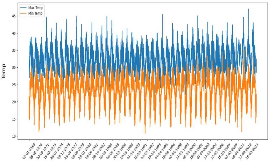
Fig.1. Temperature dataset

Fig 1 shows the plot of the complete dataset during the period under study. It's worth noting that the dataset presents inherent seasonal variations, reflecting the annual cycle of temperature changes influenced by the earth's rotation and tilt. In addition, potential longer-term trends or fluctuations in the data may mirror broader climate change trends or other macro-scale meteorological phenomena. This comprehensive dataset, with its long-term coverage and granular daily temperature records, provides a rich and detailed foundation for our comparative analysis of the XGBoost, SVM, and Random Forest machine learning methodologies in the context of temperature prediction.

4.    Methodology

The methodology adopted in this research can be broadly divided into three main stages: data pre-processing, model development, and model evaluation.

• 4.1.    Data Pre-processing

The initial stage involves pre-processing the raw data obtained from the Visakhapatnam airport meteorological station. The dataset, including daily maximum and minimum temperatures, was first cleaned and checked for any inconsistencies or missing values. Next, the following steps were executed:

• •    Normalization: Since the dataset consists of temperature values, we applied min-max normalization to scale the values between 0 and 1. This is to prevent any model from being skewed or biased due to the difference in the scale of features. Mathematically, normalization can be represented as:

  X , normalized

  
  

( X - X min )

( X - X )

( max      min )

where X is the original value, X min is the minimum value in the dataset, X max is the maximum value, and X normalized is the normalized value.

• •    Train-Test Split: The dataset was divided into training and testing sets. The training set, which included 80% of the data, was used to train the models. The remaining 20% was used as the testing set to evaluate the models' performance.

• 4.2.    Model Development

Three machine learning models were developed using the Python-based libraries XGBoost, scikit-learn's Support Vector Machine (SVM), and Random Forest.

XGBoost : XGBoost (Extreme Gradient Boosting) is a powerful machine learning algorithm that belongs to the family of gradient boosting methods. It has gained significant popularity due to its ability to deliver high predictive accuracy in various domains, including classification, regression, and ranking problems. XGBoost builds an ensemble of weak prediction models, typically decision trees, in a sequential manner, where each subsequent model corrects the mistakes made by the previous models. The algorithm aims to minimize a loss function that quantifies the difference between the predicted and actual values.

Mathematically, XGBoost can be described as follows:

Given a training dataset with N samples, each represented by a set of features X and corresponding labels y, X = {x₁, x₂, ..., x N } and y = {y₁, y₂, ..., y N }, XGBoost constructs an ensemble model F(x) by adding up a series of M weak models fₘ(x):

F ( X) = 2 f- ( *) m where fₘ(x) represents the mth weak model.

To train the XGBoost algorithm, an additive training objective is defined based on the gradient and Hessian of the loss function. For a given loss function L(y, F(x)), the objective function can be written as:

Ob ( © ) = 2 L ( y i , F ( * i )) + Z^Q ( l )

im where Θ represents the set of model parameters, and Ω(fₘ) is a regularization term that prevents overfitting by penalizing complex models. The regularization term Ω(fₘ) is typically defined as:

П( fm ) = YT + ~ X km where γ and λ are hyperparameters, T represents the number of leaves in the model, and ∥wₘ∥² denotes the L2 regularization term.

To build each weak model fₘ(x), XGBoost employs a greedy algorithm that optimizes a specific objective function to determine the best split at each tree node. This objective function takes into account the gain achieved by the split and the regularization term. The gain is defined as:

1 Г ( G L ) 2

Gain = - —:--- 2 H^L + X

+ - Г (G R ^L

2 H R + X

+ -

( G L + G R )²

( H^L + H^R + X )

where Gᴸ and Gᴿ represent the sum of gradients for the left and right child nodes, respectively, and Hᴸ and Hᴿ denote the sum of Hessians. By iteratively adding weak models to the ensemble, XGBoost gradually improves its predictive accuracy by minimizing the objective function using gradient descent optimization techniques. XGBoost also incorporates additional techniques such as column subsampling (to handle high-dimensional data), row subsampling (to handle large datasets), and regularization techniques (to prevent overfitting).

Support Vector Machine (SVM): Support Vector Machines (SVM) is a powerful machine learning algorithm widely used for classification and regression tasks. SVMs are particularly effective in scenarios where the data is not linearly separable, as they can find optimal decision boundaries by mapping the data into a higher-dimensional feature space. SVM aims to find a hyperplane that maximally separates the data points of different classes. The hyperplane is defined by a subset of training samples called support vectors, which are the data points closest to the decision boundary. SVMs can handle both linear and nonlinear classification problems using different kernel functions.

Mathematically, SVM can be described as follows:

Given a training dataset with N samples, each represented by a set of features X and corresponding labels y, X = {x₁, x₂, ..., x N } and y = {y₁, y₂, ..., y N }, where y ∈ {-1, 1}, SVM seeks to find a decision function f(x) that predicts the class label y for a new input x.

The decision function f(x) is defined as:

f ( x ) = sign ( к .Ф( x ) + b )

where w is the weight vector, ϕ(x) is the feature mapping function that maps the input x into a higher-dimensional space, and b is the bias term.

Fig.2. Model development workflow

To train an SVM, we aim to find the optimal weight vector w and bias term b that minimize a cost function while maximizing the margin between the support vectors.

The cost function consists of two terms: the regularization term, which controls the complexity of the model, and the hinge loss, which penalizes misclassifications. The cost function can be written as:

min1

w | |² + C Z max(0,1 - y, ( w .Ф( x, ) + b ))

where C is the regularization parameter that determines the trade-off between achieving a smaller margin and incurring more misclassifications.

To handle nonlinearly separable data, SVM employs the kernel trick. The kernel function K(x, x') computes the inner product between two data points in the higher-dimensional feature space without explicitly calculating the transformation. Popular kernel functions include the linear kernel, polynomial kernel, radial basis function (RBF) kernel, and sigmoid kernel.

Random Forest : Random Forest is a powerful ensemble learning algorithm that combines multiple decision trees to make accurate predictions. It is widely used for classification, regression, and outlier detection tasks. Random Forest leverages the principle of "wisdom of the crowd" by aggregating the predictions of individual decision trees to produce the final prediction.

The algorithm operates by constructing a multitude of decision trees using bootstrap aggregating (or bagging) and feature randomization. Bagging involves randomly sampling the training data with replacement to create multiple subsets, and then training each decision tree on a different subset. Feature randomization, on the other hand, involves randomly selecting a subset of features at each split within each tree.

Mathematically, Random Forest can be described as follows:

Given a training dataset with N samples, each represented by a set of features X and corresponding labels y, X = {xi, X2, ..., xN} and y = {yi, y2, ..., yN}, Random Forest constructs an ensemble model F(x) by combining the predictions of M decision trees:

F ( x ) = T7 Z f m ( x )

Mm where fm(x) represents the mth decision tree.

To train the Random Forest algorithm, each decision tree is built as follows:

• •    Randomly select a subset of the training data using bootstrap sampling.

• •    Randomly select a subset of features at each split.

• •    Create the decision tree by recursively splitting the data based on the selected features and their optimal split points.

• •    Repeat steps 1-3 for each decision tree until the desired number of trees is reached.

• 4.3.    Model Evaluation

During prediction, each decision tree in the Random Forest independently produces a prediction, and the final prediction is determined by aggregating the individual predictions through majority voting (for classification) or averaging (for regression).

The models were trained using the training data, with model hyperparameters optimized using a grid search approach to enhance performance.

The models were evaluated using several popular evaluation metrics for regression problems. Each of these metrics provides a unique perspective on the model's performance and are essential for a comprehensive understanding of each model's strengths and weaknesses.

Mean Absolute Error (MAE) : The Mean Absolute Error is an intuitive metric that measures the average magnitude of the errors in a set of predictions, without considering their direction. It's calculated as the average absolute difference between the predicted and actual values. The mathematical representation is:

n

MAE=1∑y-yˆ n1

where y is the actual value, ŷ is the predicted value, and n is the number of observations.

Mean Squared Error (MSE) : The Mean Squared Error measures the average of the squares of the errors—that is, the average squared difference between the estimated and actual values. This metric gives a higher penalty to large errors. It is given by:

n

MSE =

¹ ∑ ( y - y ˆ)² n 1

where y is the actual value, ŷ is the predicted value, and n is the number of observations.

Root Mean Squared Error (RMSE) : The Root Mean Squared Error is simply the square root of the mean square error. It measures the standard deviation of the residuals. The RMSE amplifies and severely punishes large errors. The mathematical formula is:

n

RMSE =

¹ ∑ ( y - y ˆ)²

n 1

where y is the actual value, ŷ is the predicted value, and n is the number of observations.

R2 Score (Coefficient of Determination) : The R2 score represents the proportion of the variance in the dependent variable that is predictable from the independent variables. It provides an indication of goodness of fit and therefore a measure of how well unseen samples are likely to be predicted by the model. The formula for R2 score is:

^SS res

R2=1-SStot where SSres is the sum of squares of residuals and SStot is the total sum of squares.

Mean Absolute Percentage Error (MAPE) : The Mean Absolute Percentage Error measures the size of the error in percentage terms. It is calculated as the average of the unsigned percentage error, as shown below:

MAPE =

100 ⁿ y - y ˆ n ∑ 1    y

where y is the actual value, ŷ is the predicted value, and n is the number of observations.

Explained Variance Score : The explained variance score measures the proportion to which a mathematical model accounts for the variation (dispersion) of a given data set. It is calculated as:

EVS =

^{Var ( y} true ^{- y} pred ⁾

Var ( y_true )

where Var is the variance, y true is the actual value, and y pred is the predicted value.

The model's performance was evaluated by comparing the predicted values against actual observations of the maximum and minimum temperatures, which are presented in Fig 3. It is worth noting that the predictions were made on test data, which was not used during the model's training phase.

5.    Results

In the comprehensive evaluation of the three machine learning models—XGBoost, Support Vector Machine (SVM), and Random Forest—we scrutinized their performance based on various metrics: Training Loss, Mean Absolute Error (MAE), Mean Squared Error (MSE), Root Mean Squared Error (RMSE), R2 Score, Mean Absolute Percentage Error (MAPE), and Explained Variance Score. These metrics were carefully chosen to provide a holistic and well-rounded assessment of the predictive performance of each model on the 45-year daily maximum and minimum temperature dataset of Visakhapatnam airport. Table 2, Table 3 and Table 4 show the evaluation metrics recorded by using different models – XGBoost, SVM and Random Forest respectively.

For maximum temperature predictions:

• •    XGBoost achieved a reasonable performance, with an RMSE of 0.0696, suggesting an average deviation of approximately 0.0696 degrees Celsius between the predicted and actual maximum temperatures. The R2 score of 0.717 indicates that around 71.7% of the variability in the maximum temperature can be explained by the XGBoost model. The MAE of 0.0487 implies an average absolute difference of 0.0487 degrees Celsius, while the MSE of 0.0048 represents the average squared difference between the predicted and actual values.

• •    SVM outperformed XGBoost, demonstrating better predictive accuracy with an RMSE of 0.0640, indicating a lower average deviation between the predicted and actual maximum temperatures. The R2 score of 0.760 suggests that approximately 76.0% of the variance in the maximum temperature can be explained by the SVM model. The MAE of 0.0450 indicates a lower average absolute difference compared to XGBoost. The MSE of 0.0041 represents the average squared difference between the predicted and actual values.

• •    Random Forest achieved performance similar to SVM, with an RMSE of 0.0646. The R2 score of 0.756 suggests that approximately 75.6% of the variability in the maximum temperature can be explained by the Random Forest model. The MAE of 0.0449 and MSE of 0.0042 indicate slightly lower absolute difference and squared difference, respectively, compared to both XGBoost and SVM.

Table 2. Evaluation metrics for XGBoost

Metric	Maximum Temperature	Minimum Temperature
Training loss	0.0012793670190659303	0.0011861501407973577
MAE	0.04866460745544329	0.0491364995560257
MSE	0.004839716746530099	0.004441840356037088
RMSE	0.06956807275273694	0.06664713314192207
R2 score	0.7170330669411042	0.8312993652047881
MAPE	10.884685918984946	10.180267310219527
EVS	0.7229018585315727	0.8313413678443901

— Actual Temperature

— Predicted Temperature

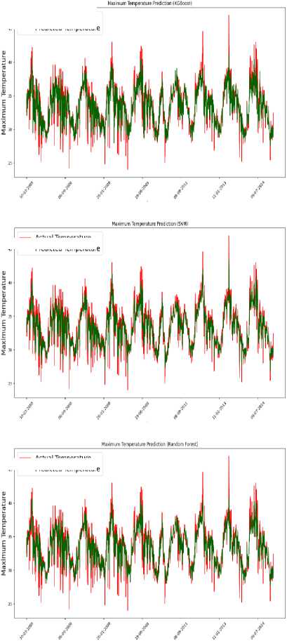
— Actual Temperature

— Predicted Temperature

— Actual Temperature

— Predicted Temperature

Minimum Temperature Prediction IXSBoostl

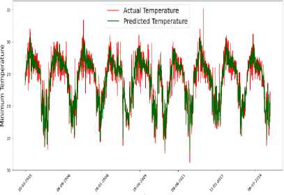
Minimum Temperature Prediction C5VMI

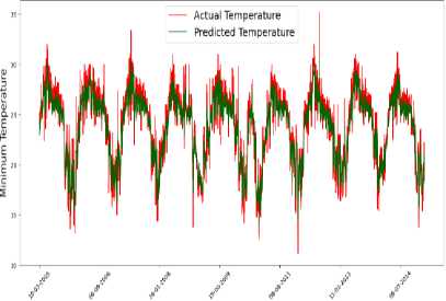
Minimum Temperature Prediction I Random ForeMI

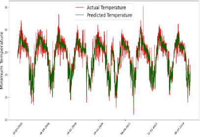
Fig.3. Temperature predictions by models

Table 3. Evaluation metrics for SVM

Metric	Maximum Temperature	Minimum Temperature
Training loss	0.004080078950598655	0.0042515573456943685
MAE	0.045008317230289675	0.05026743363944777
MSE	0.004101403925432425	0.004403685403113973
RMSE	0.06404220425182464	0.06636026976372213
R2 score	0.7602004929632691	0.8327484863489018
MAPE	10.144323506504707	10.500680210875403
EVS	0.7662323702976535	0.8380080555954982

Further examination of the results reveals that SVM and Random Forest models exhibit similar performance in predicting the maximum temperature, with slightly lower errors compared to XGBoost. This suggests that both SVM and Random Forest are effective in capturing the underlying patterns and trends in the maximum temperature dataset.

For minimum temperature predictions:

• •    XGBoost performed reasonably well with an RMSE of 0.0666, implying an average deviation of approximately 0.0666 degrees Celsius between the predicted and actual minimum temperatures. The R2 score of 0.831 suggests that around 83.1% of the variability in the minimum temperature can be explained by the XGBoost model. The MAE of 0.0491 suggests an average absolute difference of 0.0491 degrees Celsius

  between the predicted and actual values. The MSE of 0.0044 represents the average squared difference between the predicted and actual values.

• •    SVM demonstrated strong performance in predicting minimum temperatures with an RMSE of 0.0664, indicating a lower average deviation. The R2 score of 0.833 suggests that approximately 83.3% of the variability in the minimum temperature can be explained by the SVM model. The MAE of 0.0503 indicates a slightly higher average absolute difference compared to XGBoost. The MSE of 0.0044 represents the average squared difference between the predicted and actual values.

• •    Random Forest exhibited the best performance among the models, with an RMSE of 0.0640. The R2 score of 0.844 suggests that around 84.4% of the variability in the minimum temperature can be explained by the Random Forest model. The MAE of 0.0473 and MSE of 0.0041 indicate lower absolute difference and squared difference, respectively, compared to both XGBoost and SVM.

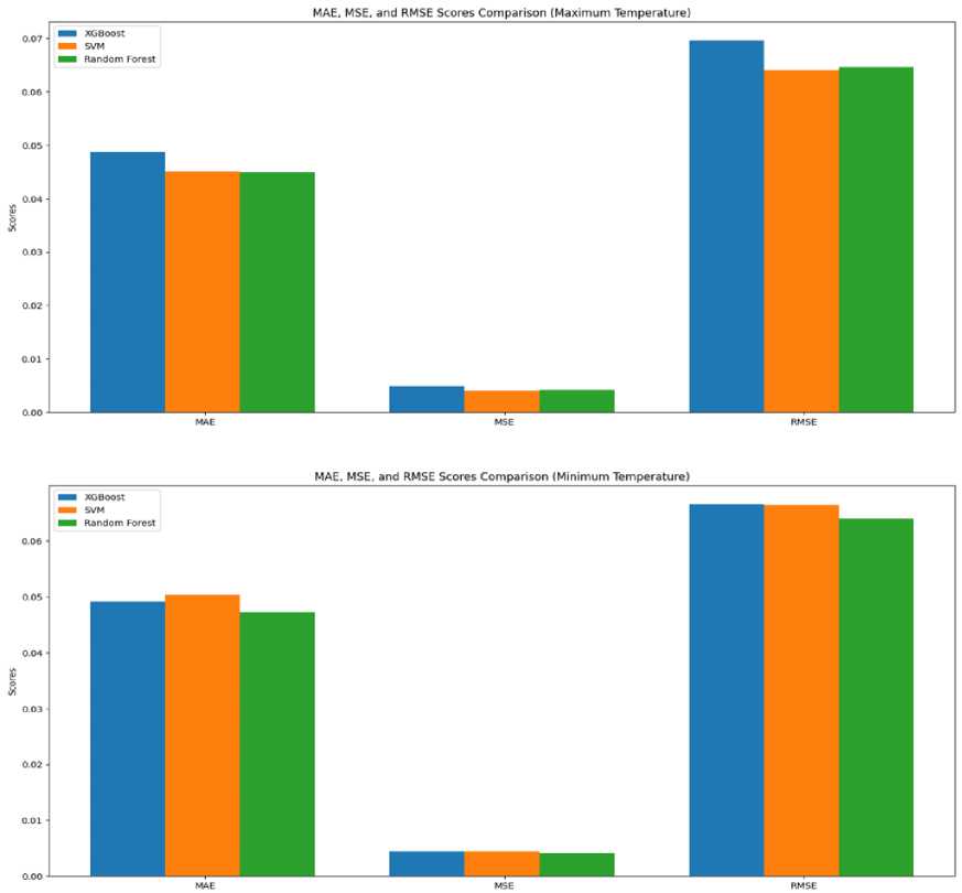
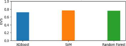
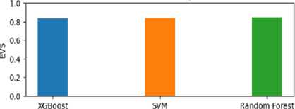
In terms of visual representation, we can examine the evaluation metrics for the three different models through the utilization of Fig 4 and Fig 5. In Fig 4, we can observe the Mean Absolute Error (MAE), Mean Squared Error (MSE), and Root Mean Squared Error (RMSE) values for the three models. When considering the maximum temperature, it becomes evident that the Support Vector Machine (SVM) model exhibits the best performance, followed by the Random Forest model and the XGBoost model. However, for the minimum temperature, the Random Forest model demonstrates superior performance, followed by the XGBoost model and the SVM model. Likewise, by referring to Figure 5, we can conduct a parallel examination that offers valuable insights into the Mean Absolute Percentage Error (MAPE), R-squared (R2), and Explained Variance Score (EVS) for the three models.

Table 4. Evaluation metrics for random forest

Metric	Maximum Temperature	Minimum Temperature
Training loss	0.0005668097065319637	0.0005530913456029689
MAE	0.04490977712627198	0.04726798594465778
MSE	0.004178151129880357	0.004098165245246876
RMSE	0.06463861949237744	0.06401691374353247
R2 score	0.7557132631932529	0.8443521101722705
MAPE	10.166482799181004	9.850708393602849
EVS	0.7596629449726479	0.8445281068761565

Upon further consolidated examination of the results, it is noteworthy that SVM consistently outperformed XGBoost in predicting both maximum and minimum temperatures. SVM achieved lower errors (RMSE and MAE) and higher explanatory power (R2 score) compared to XGBoost in both cases. This suggests that SVM's ability to construct hyperplanes in a multidimensional space, separating different classes, effectively captures the complex relationships between input features and temperature outcomes. On the other hand, Random Forest exhibited competitive performance, demonstrating similar accuracy to SVM in predicting both maximum and minimum temperatures. Although SVM outperformed Random Forest marginally in terms of RMSE and MAE for maximum temperature, Random Forest achieved the lowest errors for minimum temperature predictions. This suggests that Random Forest's ensemble of decision trees effectively captures the non-linear relationships and interactions among input variables, enabling accurate temperature predictions.

The superiority of Random Forest in predicting maximum and minimum temperature can be attributed to its ability to capture the subtle dependencies and interactions in the dataset, which play a significant role in determining minimum temperatures. Additionally, the robustness of Random Forest against noise and outliers, as mentioned in the literature review, contributes to its consistent performance.

While SVM and Random Forest demonstrated superior performance in temperature prediction, the choice of the most suitable model depends on several factors, including the specific nature of the data, the prediction task at hand, and the computational resources available. Therefore, researchers and practitioners should carefully consider these factors when selecting the most appropriate model for their specific temperature prediction needs. Also, it is crucial to acknowledge that all three models showcased competitive performance throughout this experiment, thereby demonstrating their effectiveness. Moreover, it is paramount to interpret the evaluation metrics, such as RMSE, MAE, R2 score, and MSE, in the context of the application requirements and domain-specific considerations.

In a concise manner, it can be stated that SVM and Random Forest demonstrated superior performance in predicting both maximum and minimum temperatures compared to XGBoost. Random Forest exhibited the lowest RMSE for both maximum and minimum temperatures, indicating its effectiveness in capturing the underlying patterns and trends in the temperature dataset.

These results emphasize the potential of machine learning models, particularly SVM and Random Forest, in improving temperature predictions and aiding in various domains that rely on accurate temperature forecasting.

МАРЕ for Maximum Temperature 100 T-----------------------------------------------------

80- ш 60 - i 40-

MARE for Minimum Temperature 100 ------------------------------------------------ so ■ ш 60 -

1 40-

20-

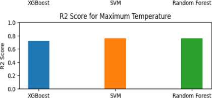
EVS for Maximum Temperature

го

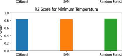
EVS for Minimum Temperature

6.    Conclusions

In conclusion, this study examined the performance of three advanced machine learning models, namely XGBoost, Support Vector Machine (SVM), and Random Forest, in predicting daily maximum and minimum temperatures using a 45-year dataset from Visakhapatnam airport. The results showed that all three models achieved relatively low training loss, indicating their ability to capture patterns in the temperature data. The MAE, MSE, RMSE, R2 score, MAPE, and explained variance score were used as evaluation metrics to assess the models' predictive performance. For maximum temperature prediction, all three models performed reasonably well, with SVM and Random Forest showing slightly better performance across several metrics. Similarly, for minimum temperature prediction, SVM and Random Forest demonstrated competitive results, while XGBoost performed adequately. These findings highlight the potential of machine learning models in enhancing temperature forecasting accuracy. The use of advanced algorithms allows for improved understanding of complex, nonlinear weather patterns, enabling better predictions and aiding in the development of effective climate change mitigation and adaptation strategies. The scientific justification for this work lies in the need for accurate temperature predictions, which have wide-ranging applications across various sectors, including agriculture, energy, transportation, and urban planning. By improving our understanding of complex, nonlinear weather patterns and enabling more precise temperature forecasts, this research supports the development of effective climate change mitigation and adaptation strategies. Further research could explore the incorporation of additional features or the use of ensemble methods to further enhance temperature prediction accuracy. Additionally, investigating the performance of these models on different geographic locations and climatic conditions could provide valuable insights into their generalizability and applicability across diverse contexts. Finally, this study advances the field by demonstrating the effectiveness of machine learning models in temperature prediction, providing scientific justification for their utilization in practical applications. The identified models and evaluation metrics offer valuable guidance for researchers and practitioners seeking to improve temperature forecasting capabilities. The study's outcomes contribute to the ongoing efforts to harness the power of machine learning in meteorology and supp ort evidence-based decision-making processes across various domains dependent on accurate temperature predictions. The results obtained from this study can serve as a foundation for future work in this field and support decision-making processes in various sectors that rely on accurate temperature predictions.