Mathematical model of the mirror system of the Millimetron observatory and a description of the method of pre-measurement of the telescope within this model

Introduction. One of the main directions for the development of onboard space technology is the creation of multi-zone high-aperture mirror telescopes that ensure the collection and processing of information in the range of radiation spectrum from X-ray to millimeter. An example of this is the draft Space Observatory "Millimetron" (Spektr-M), calculated for operation in millimeter and far IR ranges (70 μm - 10 mm) with a 10-meter cooled (~ 4.5 K) cryogenic telescope [1-3]. The main problem of creating large telescopes is to ensure the quality of the image, which in turn requires the development of high-quality and high-precision methods for monitoring the form of composite elements of their mirror system [4-6]. In [7] an overview of the state and trends in the development of space telescreen abroad is presented. The results of the work carried out in a number of leading countries in the design and construction of optical observation systems of space are set out. Large optical telescopes with composite and flexible mirrors managed by active systems are considered in orbit, to eliminate deformations at all stages of manufacturing and operation.

Creating various monitoring systems for the form of composite elements of such telescopes requires the development of mathematical models and algorithms for the operation of the control systems [8-16]. In particular, in [8], the model of the process of adjusting the composite mirrors of high-aperture telescopes is set. On the basis of the introduced concept of a difference surface using the developed algorithms for the geometric and optothechnic positioning of the mirror segments, relations were obtained to estimate the accuracy of the adjustment mirrors. In [16] are briefly presented methods of adjustment and calibration of information and measurement systems on board the spacecraft of optical-electron and radio-electronic observation.

The system of controlling the mirror system of the Millimetron Observatory (SC MS) is described in this report and have no analogues of the mathematical model and its work algorithms are created to work as part of the onboard complex of the Scientific Equipment of the Millimetron Observatory and is calculated to work in the conditions of outer space. SC MS is designed to control the quality of the mirror system (MS) of the cosmic telescope and the use of data obtained by the SC MS as a feedback signal for pre-configuration and adjustment of the optical telescope system in outer space. In [17], it was described on the basis of the created mathematical model modelling the operation of the on-board 3D scanner with a preliminary measurement of the mirrors of the Millimetron Observatory using optical control marks on the surface of the mirrors. This report is devoted to the description and analysis of the possibilities of the mathematical model used in the SC MS.

Basic provisions and requirements. The optical scheme of the mirror system of the observatory (telescope) "Millimetron" is shown in Fig. 1.

The telescope can be represented as a physical model consisting of a plurality of optical reflective surfaces (RS) with a stable form. The totality of all RS of the telescope is called a mirror telescope system (MS). Examples of such RS are (see Fig. 1): secondary mirror (SM); switching mirror (SwM); any of the panel (fragments) of the multi-element paraboloid of the main mirror (MM).

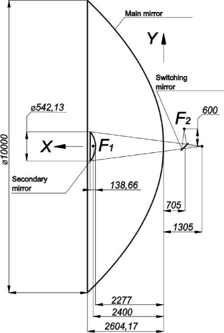
Рис. 1. Оптическая схема зеркальной системы обсерватории «Миллиметрон». Расчетные характеристики: Главное зеркало (ГЗ) – параболическое: радиус кривизны при вершине R ГЗ = 4800 мм; диаметр главного зеркала D ГЗ = 10000 мм. Вторичное зеркало (ВЗ) – гиперболическое: R ВЗ = – 254,7337 мм; D ВЗ =542,13 мм. Расстояние между ГЗ и ВЗ – 2277 мм. Эквивалентное фокусное расстояние – 70000 мм. Расстояние от ВЗ до фокальной плоскости – 3582 мм. Квадрат эксцентриситета ВЗ е² =1,147452

Fig. 1. Optical diagram of the Millimetron Observatory mirror system. Estimated characteristics: Main Mirror (MM) - parabolic: curvature radius at the top of the R MM is 4800 mm; The diameter of the main mirror of the D MM is 10,000 mm. Secondary mirror (SM) - hyperbolic: R SM - 254.7337 mm; Distance between MM and SM - 2277 mm. Equivalent focal length - 70,000 mm. Distance from SM to focal plane - 3582 mm. Square of the eccentricity of the SM e² =1,147452

The global frame of reference (GFR) of the telescope is determined by the position of the coordinate origin and coordinate axes. The top of the paraboloid of the main mirror (MM) is taken for the beginning of the GFR, in the assumption of the ideal form of the paraboloid MM. The X GFR vector is directed along the axis of the paraboloid of MM from its vertex in the direction of the secondary mirror (SM). The Y axis vector from the centre of the switching mirror (SwM) towards the focus of the receiver, indicated as F 2 in Fig. 1. The Z axis uniquely complements the X, Y axes, forming the full orthogonal basis from the vectors X, Y, Z GCS, in which the GFR is the right coordinate system.

The unambiguous position of each RS as the surface of the solid object in space is determined by:

– selected base point on a solid object containing RS . The position of this base point of the object is determined by its coordinates in GFR.

– three angles of rotation of the object with the RS relative to its base axes in GFR (Euler angles).

As a result, the position of each RS in the telescope model is set to 6 parameters - three angles of rotation of the object, and then the radius-vector displacement of the base point of the object in GFR.

Knowledge of the position of each RS telescope according to its (6 or other sufficient quantities) own parameters (degrees of freedom) means that the geometry (or configuration) of the entire MS of the telescope is accurate and uniquely defined within this model. In this case, it is possible to estimate optical quality of the telescope and its subsequent setting.

Denote a complete set of parameters describing the position of all telescope RS as a vector (parameter set) X . Vector components contain all the parameters of each telescope RS in its specified state. For example, if we used in the design only 3 RS, each described by the 6th parameters, then the vector X would consist of 18 values.

The measurement of the surface of the telescope with the 3D scanner, which is a regular element of the SC MS, is indirect, since it does not directly measure parameters of the vector, but measures the geometric magnitudes available for measurement, associated with the vector. Therefore, the task of SC MS is the definition of the vector of unknown parameters for indirect measurements obtained by the 3D scanner telescope. To obtain indirect information about the geometry of the telescope in the SC MS, a 3D scanner is laid. The 3D scanner is a device located in the "warm compartment" of KA, which can run a thin measuring (optical) beam in the MS of the telescope through the temporary optical window between the "warm compartment" and the "cold zone" and "observe" for all RS from the point F2.

Optical control marks (CM) are located on the surfaces of the RS, which can be measured by a 3D scanner beam. CM is a metal ball (or a spherical mirror, with a characteristic diameter of at least 10 mm).

The 3D scanner consists of:

– a distance measurement channel (DMC), which allows to measure the length of the optical path between the input pupil of the receiving-transmitting lens of the DMC and some CM of the RS. To do this, the measuring beam is sent through the sequence of RS, the reflection back is recorded and the optical distance between the 3D scanner lens and CM is calculated;

– the scanning mirror (ScM) of the 3D scanner, which specifies the direction of the measuring beam of the DMC for aiming to the centre of the selected CM.

The operation of the SC MS is as follows:

– measurement of all or a subset of CM using a 3D scanner is performed. For each measured CM at the outlet of the 3D scanner, 3 measurement channels are formed (with indices m = 0,1,2): m=0 - the length of the optical path of DMC to CM; m=1,2 - two angles ScM with an accurate aiming at CM.

– as a result of the measurement of the set of CM on MS, a set of measurements is obtained (three dimensions for each CM), which is indicated by the vector Y ;

– the known (after a set of a set CM) vector Y the known (after a set of a set CM) vector will be used to evaluate and restore the vector of unknown telescope parameters X .

The mathematical model described below gives an idea how to associate implicit measurements of CM (optical CM) Y with unknown parameters of the RS of the telescope X .

Mathematical model.

The positions of all RS are determined by the vector of unknown parameters X .

Let the total number of unknown telescope parameters on all RS (vector length X ) is equal to P . Individual parameter index: p = 0,..., P — 1 . In this case, the specific value of the parameter from the set X = { x_p } with the selected index p is indicated as: x_p .

Since the provisions of the CM are associated with the position of the RS, then we can enter the measurement function of the 3D scanner of the position of the CM with an index k , through the measurement channel m from the vector of the telescope status X as:

^fm , k ^{( X )} = ^fm , k ( ^X 0 , ^X1,-^XP — 1 )

Measuring with the 3D scanner of all tags forms a known vector Y ( x ) = { f_m Дх ) } .

The vector Y (the set of all measurements of the CM on all channels of the 3D scanner) depends on the vector X (all unknown parameters of the RS). Measurement functions f_{m k} = f_{m 4}( X ) = f_m (X x ₀, X j,... x_p _J depending on X are substantially nonlinear and are determined by drawings and the current telescope geometry.

Since when withdrawing the space observatory in orbit and after the disclosure of the telescope into the working position, its geometry is distorted slightly in relation to its linear and other sizes, then nonlinear functions f_{m k} ( ) can be considered constant with respect to a SMALL change in the argument X , describing the state of the MS of the telescope, which has been confirmed by numerical experiments.

In this case, the functions f_{m k} ( ) can be considered known and calculated by the initial design of the telescope in the configured state (based on geometric data from the design documentation (DD) of the telescope).

As a result, we have the following:

– the position of the telescope is uniquely determined by the unknown vector X ;

– 3D scanner SC MS can measure the position of the CM (optical control marks) which are described by the functions ^f _m , k ^{( x )} ;

• - functions f_{m k} ( ) are known (calculated according to the drawings of the DD) and are assumed to be constant (independent of the small change of argument X ).

Based on these assumptions, we will solve the opposite task, that is, we define the disorder of the parameters of the RS ( X ) from their initial (ideal) position according to the results of the implicit measure of the set of CM ( Y ) using 3D scanner.

Problem statement.

Let the telescope is configured, it corresponds to the configured position of all its RSs , which we denote as a vector X = { ~ } , consisting of parameters ~. The parameters ~ of the configured telescope can potentially be measured in the factory conditions, but this information is not needed as shown below.

With the configured state of the telescope SC MS performs the measurement of all its CM k = 0,

...

, K - 1 using a 3D scanner on all 3D scanner measurement channels m = 0,1, 2 . An array of initial

measurements Y = { f_{m k} } (for a configured telescope on Earth) is created, which corresponds to the configured vector of the parameters X ~ of the MS:

f„ J. = f. , k ( X ) = f m , k ( ~ 0 ,.~„...,~ P - . ) ^Y = { f mk ^{( X )}} •

An array of measurements of a configured telescope Y ~ is remembered. After withdrawing a telescope into orbit and its disclosure in the working position, the MS of the telescope is unbalanced, therefore, in the new position of the telescope in the orbit, its parameters of the RS X = { X_p } are accidentally offset with respect to the original (configured) state X = { x } :

x₀ = x₀ + A x ₀

X [ = X [ + A x!

~ or X = X + x,

...

X _P - 1 = ~ _P । + A x _p 1

, where x = {Ax}= {Xp - x } - is the difference vector of the displacement of the parameters of the RS. The smallness of displacements x = {Ax} = {Xp - xp } is relied.

After measuring the 3D scanner of the SC MS of all CM in orbit, we get a new set of measurements of the CM position Y = ^{f m , k ^{} :}

f m , k = f., ( X ) = f m , k ( X o , X„- X p - , ) .

The difference between the obtained sets of measurements in orbit Y =

{ f_{m k} } and confined in the factory

conditions Y = { f_{m k} } may be linearly approximated (through the differential of the multidimensional function or multi-dimensional Taylor expansion) [18] as:

ˆ~ fm, k — fm, k   fm, k

where d

m , k , p

_ ^{d f}m , k ^{( X}0 , ^X 1

5 ^x о

-1 ,... ^xp _— 1 )

•A x о + ... +-- • A x

5 ^x p - 1

■ p - 1 ,

5 X p

is the private derivative of the 3D scanner measurement function;

configured; y = Y - Y = { A ^fm , k } = ^{{ f} ,

—

f™ к } — vector change in all positions CM of 3D scanner.

In the matrix recording, the expression of the interconnection of measurements and changes to the parameters will be as follows:

(^f л f0,0 f d0,0,0 d0,0,1 ...    d0,0, P—1 Afu d0,1,0 d0,1,1 ...     d0,1, P—1 Af0,... d0,..., 0 d0,...,1 ...     d 0,..., P—1 Af0,K—1 d0,K —1,0 d0,K—1,1 ...   d0,K—1,P—1 Af,0 d1,0,0 d1,0,1 ...     d1,0,P—1 f Ax о ) Af,1 d1,1,0 d1,1,1 ...     d1,1,P—1 Ax1 Af,... = d1,..., 0 d1,...,1 ...      d1,..., P—1 • ... Af ,k-1 d1,K —1, 0 d1,K —1,1 ...   d1,K —1,P—1 .Axp—1J Af2,0 d2,0,0 d2,0,1 ...    d2,0,P—1 Af2,1 d2,1,0 d2,1,1 ...     d2,1,P—1 ... d2,..., 0 d2,...,1 ...     d 2,..., P—1 .Af2,к—1j . d 2, K—1,0 d 2, K—1,1 ...   d 2, K—1, P—1 > or y = H • x,

where x = { A x } = X — X is an unknown vector of displacement of parameters of all RS, which must be restored; y = ^{{ a} f m , k ^} = Y - Y – vector difference of measurements CM (in orbit with respect to measurements in a tuned telescope on earthly conditions); H = \^_тк}_P\ - calculated matrix of private derivatives, connecting the measurements of the CM and unknown parameters of the model of the MS telescope (hereinafter - the design matrix).

We reformulate the task as follows: Determine the changes in the position of the RS from the perfect configured x = { A x } = X — X CM in orbit from their perfectly configured y = { A f „ } = Y — Y .

At the same time, a matrix dependence (direct task) y = H • x is known, where H - the permanent design matrix (6) calculated according to the drawings (6). It is necessary to solve the opposite task: x = x ( H , y ) .

Problem solution.We define the vector of the primary parameters (offsets) of the MS telescope.

Primary offset parameters are the parameters of the telescope that show how one or another component of the MS is shifted relative to its original state (when the telescope is configured in the factory): x . The ^ p 1,1

length of the vector here is determined by the number of parameters / component described by them. So p1 – the number of parameters vector x describes. Hereinafter, we will take the designation under the matrix ^ p1,1

variable ... – meaning that over the bracket is a matrix element having k rows and m columns. Thus, x – is ^                                                ^

^{k , m}                                                                                                                                                       p 1,1

a vector-column p1 length or a matrix of dimension p 1 x 1 element.

For a fully configured MS of the telescope, all parameters are not displaced, that is, equal to zero and, thus, all components of the vector x are equal to zero.

^ p 1,1

We define the measurement vector (displacements) y of the telescope, which is created when ^ n ,1

measured (performed by the SC MS) of all or subset of the CM MS of the telescope: y .

^

n ,1

We define the vector of the noise of the measurements S of the telescope, which is created when n ,1

measuring (performed by the SC MS) CM MS of the telescope: £ .

n ,1

We define the primary design matrix H , as a matrix that characterizes the model of the MS of the ^T n , p ₁

telescope and connecting the primary parameters of displacements x , the measurement vector y and noise

S n ,1

S p 1,1

of measurements £ in one equation:

n ,1

У = H 1 " ^x 1 + ^£

^S           *^£     .

n ,1      n , p 1 p 1,1     ^{n ,1}

Matrix converting system parameters to primary parameters.

The primary offset parameters x directly relate to the RS positions, such as the MM panel, SM panel £ p 1,1

and the like. System parameters are parameters that have a generalizing nature and can affect the primary parameter groups. In essence, this is a multidimensional change of variables. Denote the system parameters as vector x . The number of system parameters or components of the vector is p . To mathematically p ,1

formalize the transformation of the generalization of the parameters, we introduce the matrix for the conversion of system parameters to the primary parameters S , such that x, = N ■ x . We have:

p i, p               ^£ 1    p 1, p p ,1

y = H, ■ x, + £ = H, ■ N ■ x + £

S        N  £ S S p1,p  p,1

’ p'—

n ,1      n , p 1   p 1,1

n ,1

n ,

n ,1

x ₁ S p 1

H ■ x + £ .

n , p p ,1 n ,1

Ч-1

H ■ N n , p1 p1, p

Therefore, the design matrix H (using system parameters) can be expressed as S = H, ■ S . n, p                                                           n, p " p 1, p the connection of measurements and system parameters can be expressed by the formula: y = H ■ x + £ . n 1 n, p p,1 n,1

In this case,

The random vector of the position change RS x can be characterized by its covariance matrix [19]

p ,1

S = S ^T, = X^xk ■ ^xm V If we believe that the parameters that make up the vector x , p , p     p , p                                                                                                                                        p ,1

are mutually

independent, have a zero average, then the covariance matrix simplifies and becomes diagonal:

S = S^T £  S'

p , p     p , p

V

^ 02

0 0 0

^ 12

...

ст² , p -1 7

,

'v- p, p where the standard deviation of an individual parameter with zero average is defined as:

^ ^v x^xk • x j   ^k = 0,

..., p - 1

Since the measurements of different CM are always independent of each other, the measurement of noise vector with a 3D scanner ε has a diagonal covariance matrix

G n,1

Y o

Y = YT g n,n      n,n

—

/ 1

...

,0

/ n - 1 7

,

—--------------------------V--------------------------- n,n consisting of vectors of standard measurement deviations у , where Y — V(^ ' ^) ' n,1

So, if there are two CM, closely located in the MS, then they have a similar value (almost the same) systematic errors in the 3D scanner channels, when measuring them. In this case, the use of differential measurements of CM, i.e. the pairwise difference between distances or angles of the 3D scanner channels to these CM will significantly reduce the systematic error of measuring distances or 3D scanner angles.

To formalize such a transformation in general (as a linear measurement combination), we introduce the primary measurement conversion matrix D .

m , n

We obtain a new replacement of variables, changing primary measurements y into differential u , as g             G n,1                                   m,1

u = D • y .

g  g G m,1    m,n n,1

We introduce an equivalent design matrix G of system parameters with differential dimensions:

m , p

G = D • H . Then u = G • x + X , where the equivalent noise of differential measurement X is

G G G         G G G G ’           1                                 G m,p    m,n n,p                   m,1    m,p p,1 m,1                                                                                               m,1

expressed through the initial noise of the primary measurement £ as X = G • G n,1      m,1    m,n n,1

^——^V— ^- λ

G m,1

The differential noise covariance matrix can be expressed as:

Г )

U = U ^T = cov l X

G G I G m , m m , m        \ m ,1 /

= cov I D • £

I G G \ m , n n ,1 7

Г )

= D • cov I £

G     IG m, n       \ n ,17

D ^T = D • Y • D ^T

G1 G G G1

n , m     m , n n , n  n , m

Solution of the inverse problem.There is an equation u = G • x + X , that connects unknown systemic displacements of the

1      g g G G m,1    m,p p,1

parameters of the MS x with calculated (known) differential dimensions of the CM u . In this case, the p,1

m ,1

equivalent design matrix G - is calculated (known) according to known D and G , where X - the m,p

m,n          n,pm modified vector of the noise of differential measurements. It has well-known statistical properties, such as zero mean and calculated (known) covariance matrix U = UT = D • Y • DT . Let us recall that S - a well- v     7               G  ‘^G  G G ^G m,m    m,m    m,n  n,n n,m                            p,p known covariance matrix of the scattering of unknown parameters of the RS x , which characterizes their p,1

initial scatter / disorder of the MS.

According to known: u , G , U , S it is necessary to find the most accurate solution of the equation m,1   m,p   m,m   p,p u = G • x + X , that is, to find the vector of unknown system parameters x .

v v v v ’      ’                              J     Г          v

m ,1 m , p  p ,1     m ,1

p ,1

To solve the problem we are looking for a matrix solver (matrix) F such that the assessment x of the

p,m unknown vector of system parameters x on differential measurements u is

p ,1

m ,1

p ,1

x = F • u v v v p ,1 p , m m ,1

When searching for matrix F , it is necessary to pick it up in such a way that the deviation F = x

p , m

p ,1      p ,1

- x v p ,1

of the true offset x and its calculated estimate x ˆ was minimal in the statistical sense. We define it as:

v p,1

v p,1

J =

5x

v p,1

x - x v v p ,1 p ,1

) ^ min ,

where ||a|| = /^ a 2 - is the norm of the vector; ^ ^ - average value from random variable. k

Owning long intermediate calculations, we give the final formula for the optimal solver:

f      ) ^T

F = G • S

v p,m

v v

• G • S • G T + U

v v

V m , p p , p 7 V m , p p , p

V p , m

+

*^v  v p, m   m, m 7

V m,m

,

Analysis of parameter recovery errors

The random vector error of the recovery of unknown parameters 5x - is the difference between the true p,1

unknown vector of the system parameters of the MS state after placing in orbit x and estimate x of this p,1

p ,1

vector obtained by differential measurements using formula (16):

5 x = x - x .

v v v p ,1      p ,1 p ,1

The covariance matrix for the parameter recovery error vector 5x according to the results of calculations p ,1

is as follows:

A = cov 5 x I = Q • S • Q v       v^        v

v

V

p , p

V p ,1

v p,p

v

p , p

^v p , p

■ T + F • U • F T ,

v v *^-1

p , m m , m m , p

where

Q = F • G v  v p,p    p,mm

I ^;

p , p

I v p , p

– single diagonal dimension matrix (pxp).

If you need to recognize an error (standard deviation) of the reduction F of a specific system parameter p , m

(with an index k = 0,..., p — 1 ) x [ k ] with the use of formula (16), then the formula for this will be as p ,1

follows:

^ x [ k ] = Шм!,                                                           ⁽¹9)

p,p where A [k, k] - k — й the diagonal element of the matrix A . p,p                                                                                    p,p

Conclusion.

Thus, having solved the system of equations x = F • u and having received an estimate x of the parameter displacements vector x , it becomes known to us - how and what RS is necessary to “tighten” or shift in orbit to return them to the original factory position that corresponds to the tuned telescope.

If the degree of freedom of unknown absolute parameters X (defined by the capital letter earlier) when determining the RS, it is possible to choose a conveniently appropriate actuators of the RS (for example: the SM position is set to 6 hexapod actuators, which can be defined as unknown components of the vector X ), then it gives certain convenience. In this case, the estimated bias vector x ˆ is a vector reporting “ how much each of the RS drives is shifted from the perfect (source) position, ” and in fact, as you need to make the steps of the drive, so that the RS “got up” to the original place is considered. Thus, the calculated vector x ˆ may be direct input for the mechanisms for correcting the MS of the telescope.

The use of the described telescope setup algorithm has significant positive practical qualities:

– the smallness of changes in the position of the RS allows to reduce the task to the system of linear equations. This allows to use the methods of linear algebra and gives an accurate and only solution to the inverse problem with the projected accuracy of the algorithm;

– there is no need to know the absolute values of the parameters x for the RS;

– there is no need to know exactly the absolute position of the CM in the satellite coordinate system and their installation location on the RS. It does not require high accuracy of installing CM in the MM panel and other RS.