MATLAB/Simulink Based Study of Different Approaches Using Mathematical Model of Differential Equations

Published Online April 2014 in MECS

MATLAB is a general purpose commercial simulation package used to perform numerical and symbolic computation. Generally, it is used to solve differential equations quickly and easily in an effective manner. It also leads to a visual plot of the results [5-10]. Engineering simulation using graphical programming tool Simulink plays a vital role in understanding and assessing the operation of a system. Simulink, built upon MATLAB, is a powerful interactive tool for modeling, simulating and analyzing dynamical system; thus, forming an ideal tool for qualitative and quantitative analysis of electrical and electronic network study. It has been identified as an ideal tool for laboratory projects, and has hence been adopted for teaching a variety of courses in electrical and electronics engineering. The benefits of MATLAB and Simulink have been well documented by several workers [11-18].

The present work is an implementation of MATLAB text based description m.file, graphical programming Simulink model; and data driven modeling using MATLAB and Simulink together. The MATLAB script implementation is a text based m.file description of system under reference that can be written in any text editor. The graphical approach uses Simulink model in terms of block diagram realization for visualizing system dynamics. A Simulink model for a given problem can also be constructed using building blocks from the Simulink library. The model consists of various blocks from Simulink libraries arranged in a desired fashion, offering solution to various problems without having to write any codes.

The work presented here can be implemented to investigate the response of other similar engineering applications. One can implement the MATLAB script and Simulink model presented here as a computational project based model in circuit and system course, that can contribute to an improvement in learning and ultimately to educational success in engineering program. In this study, the same has been demonstrated by considering an example of 1st order electric system. The behavior of second order system has also been investigated for step excitation for various values of damping ratio.

The organization of the present paper involves a brief introduction, followed by Section 2 which focuses on mathematical modeling of first order system. Section 3 and Section 4 describe selection of system parameters, and response analysis of first order electric circuit using MATLAB with different approaches. Section 5 deals with various approaches for analysis of first order system using Simulink. Section 6 summarizes data driven modeling followed by result and discussion in Section 7. Section 8 describes the scope of work in diverse engineering applications; and finally, Section 9 emphasizes on implementation of work presented in this study using Scilab/Xcos as an alternative to MATLAB/Simulink; followed by a conclusion in Section 10.

Taking Laplace transform of (3) and rearranging, the system function is given as:

V c ( s )         1

V ( s )   ( sRC + 1)

( s + ~)

RC

( s + ^-) T

where T = RC is the time constant of the system.

Looking at RC circuit, current as being the output and voltage across the capacitor as state variables, the state variable representation of the RC circuit is given as:

dvc(t) dt

RC

v c ^{( -} ) ⁺

The current across the circuit is

RC

vi(t)

II. Mathematical Modeling of RC System

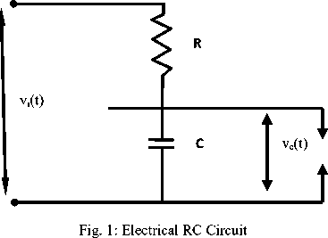
One of the first engineering applications that students always practice is first order series RC electric circuit. The differential equation governing the series RC circuit of Fig. 1 is given as:

V ^{( -} ) = I ^{( -} ) R + — l i ^{( -} d                   (1)

C where v (t) is the forcing function; v (t) is the output voltage across the capacitor; C is the capacitance of the capacitor in Farad; R is resistance of the resistor in Ohm; and i(t) is current flowing in the circuit in Ampere

The circuit current i ( t ) is given as:

dv UA i (t) = C c( ) dt

The equation (1) can be rewritten as:

RCdV c T ^- ) + V c ( - ) = V i ( - )

dt

i ^{( -} ) =

v c ^{( -} ) ⁺

R vt <-)

The matrix A B C D for RC series circuit is given as:

A =

C =

RC

- 1

B =

RC

D =

R

The mathematical model presented in this section has been implemented using MATLAB/Simulink using different approaches for chosen system parameters.

• (2)

• (3)

III. System Paramaters

In this investigation, the chosen parameters of electric circuit include: the resistance value: R =2.5 KΩ; the circuit capacitance value: C =0.002 F. The system response has been investigated for step excitation of amplitude 10, ramp function of slope 10 and impulse excitation of magnitude 10.

After setting the system parameters, the governing (3) for series RC circuit becomes:

dv ( t )

^{5         +} V c ^{( -} ) = V t ^{( -} )                            (7)

dt

Thus, the series RC circuit generates a mathematical model in terms of first order differential equation. Using the chosen design parameters, various approaches have been incorporated for deriving the solution of differential equation using MATLAB and Simulink. At first, the mathematical model presented in this section has been implemented through different approaches using MATLAB script implementation m.file.

In the 2nd part of the study, the Simulink models have been drawn directly using different approaches governing the behavior of series RC circuit. The mathematical description of the system in Simulink has been translated into block diagram representation using the various elements of Simulink block library, and finally, the solution of model has been obtained using built-in MATLAB solver.

• IV. System Response Analysis USING MATLAB

• 4.1    Symbolic Simulation Technique, Approach I (Laplace Transform Method)

In this investigation, response of first order series RC electric circuit is presented using different approaches. The effect of varying system parameters is also discussed.

In this section, MATLAB symbolic simulation technique using Laplace transform method has been employed to solve the model. The Laplace transform method (LTM) is useful for solving initial value problems involving linear constant coefficient equations. In this technique, by using Laplace transform governing, differential equations are converted into algebraic equations that can be solved by simple algebraic technique. The inverse Laplace transform is then applied to give corresponding function which forms the solution to the differential equation. The symbolic built-in commands such as 'laplace', 'ilaplace', and 'heaviside' functions have been used [5-6, 19-20].

The MATLAB script for the mathematical model of differential equation (7) using symbolic implementation is shown below in Fig. 2.

MATLAB Solution

% MATLAB script: RC1.m

%Symbolic simulation of (7) of series RC circuit clc;      % clear the command window clear all; % clear all the variables close all; %close all figure windows syms t s v %define symbolic variables v0 = 0; %define IC for v(0) vd0 = 0; %define IC for v'(0) f1=10*(heaviside(t)); %define step signal

F = laplace(f1, s); %Laplace of step input v1 = s*v - v0;      %implement Dv soltn = 5*v1+v-F; %differential equation tf=solve(soltn,v);     %solution of equations vc_output=ilaplace(tf,t); %find v(t) by using IL pretty(vc_output);

subplot(3,1,1);

ezplot(vc_output,[0,40]); % plot of symbolic object ylim([0 12])

title('Voltage versus Time for step using LTM');

xlabel('Time');

ylabel('Voltage' );

grid on

F1 = laplace(int(10*heaviside(t)),s); %LT of ramp solution1 = 5*v1+v-F1;    %implement DE tf1=solve(solution1,v);     %find sol of DE vc_output1=ilaplace(tf1,t); %find v(t)by using IL pretty(vc_output1);

subplot(3,1,2);

ezplot(vc_output1,[0,40]);

title('Voltage versus Time for ramp using LTM'); xlabel('Time');

ylabel('Voltage');

grid on

F2 = laplace(diff(10*heaviside(t)),s); %LT impulse solution2 = 5*v1+v-F2;    %differential equation tf2=solve(solution2, v);

vc_output2=ilaplace(tf2,t) ; %find v(t) by using ILT pretty (vc_output2);

subplot (3,1,3);

ezplot(vc_output2,[0,40]);

axis([0 40 0 3])

title('Voltage versus Time for impulse using LTM'); xlabel('Time');

ylabel('Voltage');

grid on

Fig. 2: MATLAB script for analysis of RC circuit (RC1.m)

• 4.1.1    Analysis using 'dsolve' commands

One can also find the solution of differential equation using 'dsolve' functions of symbolic computation. The MATLAB symbolic function 'dsolve' is used to symbolically solve the ordinary differential equations specified by ODE as first argument and the boundary or initial conditions specified as second argument. In fact, only one statement 'dsolve' is required to define the series RC circuit. The other commands are required for plotting purpose and annotation of graphical output. The MATLAB implementation to solve the (7) using 'dsolve' function is shown in Figure 3.

MATLAB Solution

%MATLAB script: RC2.m

%Symbolic solution of (7) using dsolve function clc;          %clear command window clear all;       % clear workspace close all      %close all figure windows syms t s v     % creating symbolic object out=dsolve('5*Dv+v=10*heaviside(t)','v(0)=0'); pretty(out);

subplot(3,1,1);

ezplot(out,[0,40]); % plot of symbolic objects title('Voltage versus Time for step using dsolve'); xlabel('Time');

ylabel('Voltage');

ylim([0 12]) grid on output1=int(out);         %finding ramp response pretty(output1);

subplot (3,1,2);

ezplot(output1,[0,40]);

title('Voltage versus Time for ramp using dsolve');

xlabel('Time');

ylabel('Voltage');

grid on output2=diff(out);      %finding impulse response pretty(output2);

subplot(3,1,3);

ezplot(output2,[0,40]);

title('Voltage versus Time for impulse using dsolve');

xlabel('Time');

ylabel('Voltage');

ylim([0,3]);

grid on

Fig. 3: MATLAB script using dsolve function (RC2.m)

• 4.1.2    Effect of varying the Circuit Parameters

The effect of varying the circuit parameters of first order series RC circuit has also been studied by implementing MATLAB code as shown in Figure 4. Different values of R (2, 5, 20 K Ohms) will be considered in the script presented below.

MATLAB Solution

% MATLAB script: RC3.m

% Effect of varying the circuit parameters clc;          %clear command window clear all;      %clear workspace close all;      %close all figure windows

% define circuit parameters R=2, 5 and 20 K; C=2e-3 syms t s v     % creating symbolic object v_out=dsolve('4*Dv+v=10*heaviside(t)','v(0)=0'); v_out1=dsolve('10*Dv+v=10*heaviside(t)','v(0)=0'); v_out2=dsolve('40*Dv+v=10*heaviside(t)','v(0)=0');

figure(1)

ezplot(v_out,[0 40]);

hold on ezplot(v_out1,[0 40]);

ezplot(v_out2,[ 0 40]);

axis([0 40 0 16])

xlabel('Time');

ylabel('Voltage')

legend('Step, R=2K', 'Step, R=5K', 'Step, R=20K')

title ('Voltage across capacitor for R=2, 5 and 20K are')

grid on

%voltage across resistor figure (2)

vR1=10-v_out;

vR2=10-v_out1;

vR3=10-v_out2;

ezplot(vR1,[0 40]);

hold on ezplot(vR2,[0 40]);

ezplot(vR3,[0 40]) ;

ylim([ 0 10])

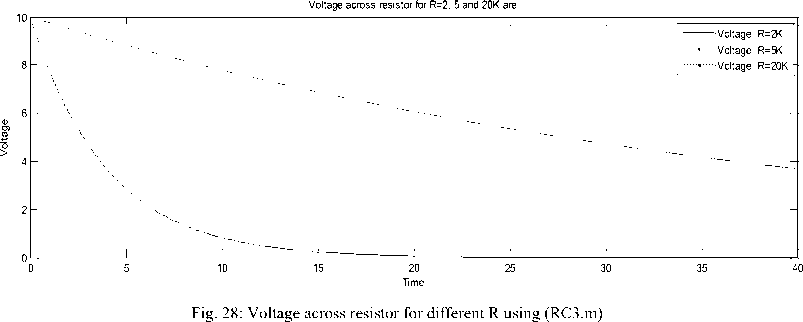
title('Voltage across resistor for R=2, 5 and 20K are')

legend('Voltage, R=2K', 'Voltage, R=5K', 'Voltage, R=20K')

xlabel('Time');

ylabel('Voltage');

grid on figure(3)

%current across resistor iR1=(10-v_out)/2e3;

iR2=(10-v_out1)/5e3;

iR3=(10-v_out2)/20e3;

ezplot(iR1,[0 40]);

hold on;

ezplot(iR2,[0 40]);

ezplot(iR3,[0 40]);

ylim([ 0 6e-3])

title ('Current i(t)for R=2, 5 and 20K are');

legend('Current, R=2K', 'Current, R=5K', 'Current,

R=20K')

xlabel('Time');

ylabel('Current');

grid on

Fig. 4: Script for varying resistance (R) (RC3.m)

• 4.2    Numerical Solution of ODEs

• 4.2.1    Simulation Using ODE MATLAB Functions, Approaches II

This section demonstrates the usage and implementation of commonly used ODE solver for solving differential equations.

In general, mathematical model of diverse engineering applications like electric circuit are designed and solved to produce the behavior of the circuit and system under different conditions. MATLAB has a library of several built-in ODE functions that can be used for particular cases. The response of electric circuit for different applied conditions has been presented here using ode45 solver. The code for a first order ODE is very straightforward. One of the features that ode45 solver requires is that the system of equations must be organized in first order differential equations. The transformation of higher ODE of the system of DE to the first ODE is mandatory. ode45 is one of the most popular code used to solve differential equations [21]. The differential equation of series RC circuit is already modeled in terms of first order differential equations as given by (7) for chosen circuit parameters.

The syntax of MATLAB ODE solver is:

[tout, yout]=solver_name (odefun, timespan, IC)

where odefun is the given DE as string contained in a m function file; time span is the range t ≤ t ≤ t     over which the solution is required

(tspan=[t0: tfinal]) and IC represents the initial conditions

The differential equation can be handled in a few simple steps.

Step1: First of all, reduce the system governing n^th order differential as a set of n first order ordinary linear or nonlinear DEs. If it is already first order, no need to convert it.

Step2: Write all the first order equation in a standard form specifying the interval of independent variable and initial value as given below.

dy

— = f ( t, y ) for   t 0 ^ t ^ t f with y = y 0 at

dt t = t о.

Step3: Create a user defined function file or use an anonymous function to solve all the first order equations for a given values of t and y. It implies that DE must be first defined in a function file.

Step4: Select a method of solution i.e. choose the built-in function of MATLAB ODE solver type.

Step5: Solve the ODE and get the result from output.

The function ode23 and ode45 are very similar. The only difference is that ode45 is fast, accurate and uses larger step sizes, but is still much slower than ode23. The response obtained using ode45 is not as smooth as using ode23. The MATLAB script for the mathematical model of series RC circuit using MATLAB ODE function is presented in Fig. 5 and 6 respectively. Fig. 5 depicts MATLAB script calling program file (RC4.m) for function file as shown in Fig.6.

MATLAB Solution

%MATLAB calling script file: RC4.m

%ODE solver approach clc;                 %clear command window clear all;               %clear workspace close all;               %close all figure windows tspan=0: 40; %define time interval to solve ODE initial =0; %define initial condition

% solve the ODE directly with ode45

[t,v]=ode45('ode3', [tspan],initial);

%plot the step response plot(t,v,'mp');

ylim([0 12]);

xlabel('Time')

ylabel('Voltage')

title('Voltage versus Time for step input using ode45') legend('Step response')

grid on

Fig. 5: Calling program file (RC4.m)

% function file that defines the DE function dydt=ode3(t,v)

% filename: ode3.m

% define model parameters

R=2.5e3; C=0.002; u=10

dydt=(u-v)/(R*C) end

Fig. 6: MATLAB ODE function script files for analysis of RC circuit

• 4.2.2    Using Anonymous Function

The solution of (7) can also be developed using anonymous function. The anonymous function can be defined in command window or be within script.

The solution applied in this study using anonymous function is coded in MATLAB program form as presented in MATLAB script m.file (RC5.m) as depicted in Fig. 7.

MATLAB Solution

%MATLAB script: RC5.m

% This program solves a system of ODE clc; %clear command window clear all; %clear workspace close all; %close all Figure windows % define electric circuit parameters R=input('Enter the resistance R:'); C=input('Enter the capacitance C:'); u=input('Enter the input signal U:');

tspan=0: 40; %define time interval to solve ODE initial =0; %define initial condition

% solve the ode directly with ODE45 ode2=@(t,v)(u-v)/(R*C);

[t,v]=ode45(ode2, tspan,initial);

plot(t,v,'r.');

ylim([0 12])

xlabel('Time')

ylabel('Voltage')

title('Step response')

legend ('Capacitor voltage') grid on

Fig. 7: MATLAB ODE script for analysis of RC circuit using anonymous function (RC5.m)

• 4.3    Simulation Using Built-in MATLAB Functions, Approaches III

• 4.3.1    The Transfer Function Method

In this section, transfer function and state space methods have been used to solve the model.

One can also study the response of electric circuit using the various built-in functions of MATLAB. The response of the RC system is investigated by subjecting the model to various chosen input functions. The system can be entered in state space form or as transfer function by means of numerator and denominator coefficient or by means of zeros, poles and the gains. Indeed, there is no direct command to obtain the ramp response of the system, therefore for obtaining ramp response the transfer function can

^G ramp ⁽ s ) = ^G step ⁽ s ⁾*1 .

be expressed as:

Finally, the ramp response

can be obtained by using MATLAB built-in function 'step'. The MATLAB script implemented to solve the RC circuit is depicted in Fig. 8.

MATLAB Solution

%MATLAB script: RC6.m

%Response of RC system using transfer function clc;          %clear command window clear all;      %clear workspace close all;               %close all figure windows

%define electric circuit parameters

R=input('Enter the resistance R:');

C=input('Enter the capacitance C:');

U=input('Enter the amplitude of step input signal U:');

num=[U]; %define the numerator of the TF den=[R*C 1];%denominator of the TF disp('The transfer function representation is:');

G=tf(num,den);% create transfer function subplot(3,1,1)

step(num,den);% plot the step response axis([0, 40, 0, 12]);

title('Step response of series RC system');

grid on subplot(3,1,2);

num1=[U];

den1=[ R*C 1 0];

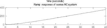
step(num1,den1)% plot the ramp response axis([0, 40, 0, 400]);

title('Ramp response of series RC system');

grid on subplot(3,1,3);

impulse(num,den);% plot the impulse response axis([0, 40, 0, 3]);

title('Impulse response of series RC system');

grid on

Fig. 8: Script for analysis of RC circuit (RC6.m)

• 4.3.2    The State Space Method

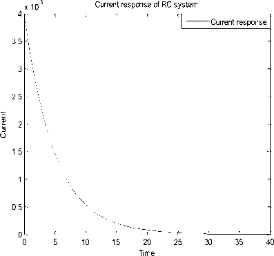
MATLAB also facilitates step response of RC system using state space approach by directly assigning system matrices/vectors as input argument [14]. The solution of RC circuit can also be developed using state space representation of (5) and (6) as depicted in Fig 9.

MATLAB Solution

%MATLAB script: RC7.m

%computes the response of RC system using SS clc;    %clear command window clear all; %clear workspace close all; %close all figure windows

R=input('Enter the resistance R:');

C=input('Enter the capacitance C:');

U=input('Enter the amplitude of step signal U:');

A= [-1/(R*C)];

B= [1/(R*C)];

C= [-1/R];

D= [1/R];

disp('The state space representation:');

G=U*ss(A,B,C,D);

step(G); % plot step response xlabel('Time')

ylabel('Current')

title('Current response of RC system')

legend ('Current response')

axis([0 40 0 4e-3]) grid on

Fig. 9: Script for analysis of RC circuit (RC7.m)

• 4.4    Analytical Computation of Time Domain Response

• 4.4.1    Computation of Time Domain Response

  • 4.4.1.1    Step Response

In this section, at first the time domain step, ramp and impulse response of electric RC circuit has been computed analytically from transfer function; and then the same has been symbolically solved using 'dsolve' command for solution of DEs. Finally MATLAB script has been developed for time domain step, ramp and impulse analytical expression.

Using (4), the system function of the circuit is given as:

G ( s ) =

V c ( s )       1

V_t ( s )    t s + 1

Laplace transform of unit step signal is

L (u ( t )) = ¹

s

Substituting the (8) in (4), the Laplace transform of output signal is

V c ( s ) =

s ( t s + 1)

Applying inverse Laplace transform, the step response of the system is vc (t) = (1 - e- t / t )for t > 0

In other words, for step input with amplitude A i.e v_t ( t ) = Au ( t ) the step response is given by v_c ( t ) = A (1 - e - t / ^t ) for t >  0 (10)

• 4.4.1.2    Ramp Response

Laplace transform of ramp signal is

L ( r ( t )) = 4

s ²

Substituting the (11) in (4), the Laplace transform of output signal is

V c ( » ) =

5 ²( 7S + 1)

Applying inverse Laplace transform, the ramp response of the system is given as:

t vc (t) = t - t(1 - e T) for t > 0

In other words, if we have ramp input with slope A i.e vi (t) = A1 r(t) the ramp response is given by vc (t) = A (t - t(1 - e"T )) for t > 0          (13)

4.4.1.3 Impulse Response

Laplace transform of impulse signal is

L (5( t )) = 1                                    (14)

t V_c ( s ) + V c ( s ) = V ( s )                      (17)

Converting (17) back to a differential equation, we get '

™c ⁽ t ) ⁺ v c ⁽ t ) = ^vi ⁽ t )                           (18)

For computing step response v_t ( t ) = 1 for t >  0

Substituting the same in (18), the governing differential equation for step signal is: '

^ v c ⁽ t ) ⁺ v c ⁽ t ) = ¹                                (19)

For computing ramp response v_t ( t ) = t for t >  0

The governing differential equation for ramp signal is:

T v c ( t ) + v_c ( t ) = t                               (20)

For      computing      impulse      response v (t) = dirac (t) for t > 0

Substituting the same in (18), the governing differential equation for impulse signal is:

tv_c ( t ) + v_c ( t ) = dirac ( t )                       (21)

Substituting the (14) in (4), the Laplace transform of output signal is

V c ( s ) =

( t s + 1)

t( s +

Applying inverse Laplace transform, the impulse response is vc (t) = 1 e -t /T for t > 0

т

In other words, for an impulse voltage input with area or strength A₂ i.e v_t ( t ) = A ^ ( t )

The Impulse response is give by

v ( t ) = -A ²- e ^- t / ^T for t >  0 c     _RC

4.4.2 Analytical Computation of Time Domain Response Using Symbolic Solution

In this part, the time domain analytical expression of the capacitor voltage v ( t ) for step, ramp and impulse excitation has been obtained by the solution of (3) using 'dsolve' function.

Using (4) and cross multiplying, the equation that describes the electric circuit is

The MATLAB script developed to compute time domain step, ramp and impulse response given by (19), (20) and (21) is developed below in Fig.10.

MATLAB Solution

MATLAB script: RC8.m

% Solution of DE using dsolve function

% Time domain step solution of DE step=dsolve('tau*Dy+y=1','y(0)=0')

% Time domain ramp solution of DE ramp=dsolve('tau*Dy+y=t','y(0)=0')

Fig. 10: Differential equation solution using dsolve function (RC8.m)

4.5 Plotting of Analytical Computation of Time Domain Response, Approaches IV

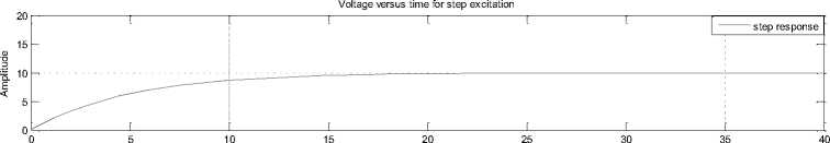
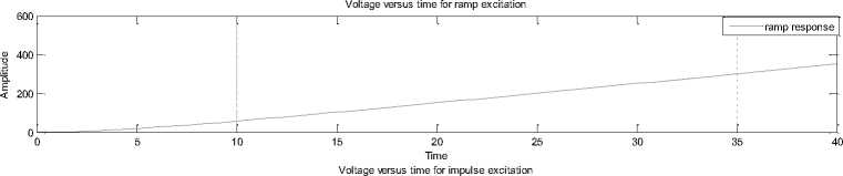
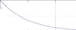
The time domain analytical expression of the capacitor voltage v ( t ) for step, ramp and impulse excitation is obtained by the solution of (3) and is given by (10), (13) and (16) respectively. The system response of electric circuit under reference has also been plotted by implementing a MATLAB script of time domain representation of (10), (13) and (16) for chosen system paramaters. A typical MATLAB solution m.file developed for time domain response plotting is depicted in Fig. 11.

MATLAB Solution

%MATLAB script: RC9.m

%plotting of analytical time domain response clc;              %clear command window clear all;           %clear workspace close all;           %close all figure windows

%define parameters of electric circuit

R=input('Enter the resistance R:');

C=input('Enter the capacitance C:');

A=input('Enter the step input amplitude A:');

A1=input('Enter the ramp input slope A1:');

A2=input('Enter the impulse input strength A2:');

T=R*C; %compute RC time constant of the circuit t=0: T/100:8*T; %create time index vector subplot(3,1,1)

v1=A*(1-exp(-t/T)); %time domain step expression plot (t, v1,'r'); % plot the variables axis([0 40 0 12]);

xlabel('Time');

ylabel('Voltage');

title('Voltage versus Time for step excitation');

grid on subplot(3,1,2)

v2=A1*(t-T*(1-exp(-t/T))); %time domain ramp response plot (t, v2,'m');

xlabel('Time');

ylabel('Voltage');

title('Voltage versus Time for ramp excitation');

grid on subplot(3,1,3)

v3=(A2/T)*exp(-t/T); % time domain impulse relation plot (t, v3);

xlabel('Time');

ylabel('Voltage');

title ('Voltage versus time for impulse excitation'); grid on

Fig. 11: MATLAB script for plotting of analytical time domain response of RC circuit (RC9.m)

• 4.6 Comparison of Symbolic dsolve Obtained Solution with a Direct Solution ODE Solver, Approaches V

This section gives a comparison of symbolic solution with analytical solution. The MATLAB script for comparing symbolic solution with direct ode45 solver is shown in Fig. 12.

MATLAB Solution

%MATLAB script: RC10.m

%solve a system of ODE using anonymous function %Solution using MATLAB ODE45 function %Symbolic solution of (7) using dsolve function clc;          %clear command window clear all;       %clear workspace close all;       %close all figure windows syms t s v     %creating symbolic object

% define parameters of electric circuit

R=input('Enter the resistance R:');

C=input('Enter the capacitance C:');

u=input('Enter the input signal u:');

out=dsolve('5*Dv+v=10*heaviside(t)','v(0)=0');

pretty(out);

ezplot(out,[0,40]); %symbolic plot of step response hold on

%solve the ode directly with ODE45

ode2=@(t,v)(u-v)/(R*C);

[t,v]=ode45(ode2,0:40,0);

plot(t,v,'r+','Linewidth',1); %plot the response axis([0 40 0 12]);

xlabel('Time');

ylabel('Voltage');

title('Voltage versus Time for step excitation');

legend('symbolic solution', 'ode solver solution') grid on

Fig. 12: MATLAB script for comparison of symbolic dsolve obtained solution with a direct solution ODE solver (RC10.m)

The forthcoming section presents the simulation and analysis of first order electric circuit using Simulink. The mathematical model of RC circuit described in section (2) has been utilized in Simulink model development, and finally, some results of simulation have been presented.

• V. System Response Analysis Using SIMULINK

Simulink is a powerful interactive simulation tool built upon MATLAB. In Simulink, a typical model consists of the source, the system being modeled and sinks. The source block provides an input signal to a system in order to extract its behavior. A system is an object or a collection of interconnected objects or block diagram representation of process being modeled whose behavior can be investigated using Simulink methods. The Simulink model is created using various blocks of library available in Simulink. The sink blocks are display devices used to visualize the output.

Engineering systems are often modeled using different approaches such as differential equation, transfer function and state space. The Simulink model can be drawn directly using different approaches governing the behavior of circuit or system under reference. Simulink converts graphical representation into a state space representation consisting of the set of simultaneous first order differential/difference equations. These equations are then solved by using MATLAB integrating functions [11-13]. The steps for Simulink solution is as follows:

Step1: Firstly, describe the mathematical model of system under reference.

Step2: Open a new Simulink model window.

Step3: Select the required number of desired blocks from Simulink library and copy into model window.

Step4: Connect the appropriate block and customize each block as desired. Save the model.

Step5: Make the required changes in the simulation parameters.

Step6: Run the simulation model and observe the result.

In the forthcoming subsection, the various approaches for solving the first order RC circuit is presented.

• 5.1    Simulation Model Using Differential Equations, Approaches I

On solving the (3), the highest derivates term is given as:

dvc(t) = J- (v (t) - v (t)) dt RC i     c

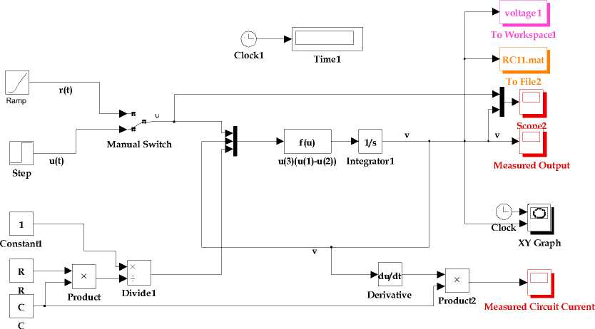
In this methodology, the differential equation governing the RC electric circuit is arranged as (22) for highest order derivates in the left side [22-27]. In order to develop the Simulink model using (22), firstly, the number of terms inside the differential equation to be solved is identified. Each term requires a series of operation. The Simulink block needed for solving differential equation (22) are dragged from respective block libraries as per requirement and interconnected to create the model. The various blocks such as signal generator, step and constant block in source library; product and subtraction block in the Simulink math library; the integrator block in Simulink continuous library and the scope, To workspace, To file, XY graph are dragged from sink block library. The integrator is the basic building blocks for solving differential equations. The Clock block generates the time and the same is copied to workspace. The Simulink model solution for first order differential equation (22) is depicted in Fig. 13. In this Simulink model, one can choose the input excitation from signal generator, ramp or impulse using multiport switch. Depending on numerical constant specified in the control port, one can select the corresponding signal. There is a provision to select multiple inputs from signal generator such as sine and square.

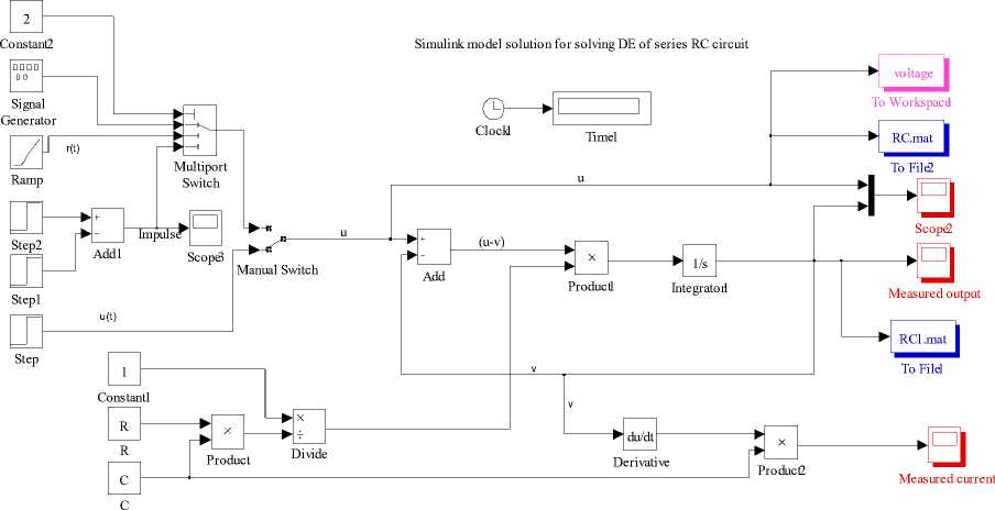
After construction of the model, all system parameters for model are set by double clicking on each block as chosen before running simulation. After customization of Simulink model, simulation is performed for specified time period to analyze its behavior. One can visualize the input and output plot on the same scope using mux block as indicated in Scope 2 of model. The 'To Wokspace' and 'To File' block is used to save the data in the Workspace and to MAT files for later processing.

• 5.2    Simulation Model Using Transfer Function, Approach II

Simulink enables to simulate continuous time system either using state space or transfer function of electric circuit forming the system using individual blocks from the Simulink continuous block library.

The transfer function of series RC circuit as given by (4) is:

V c ( s )         1

V( s )   ( sRC + 1)

( s + ”)

RC

( s + -)

T

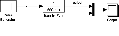
Alternatively, one can develop the Simulink model using (4) and study the behavior of RC series circuit using the various blocks of continuous blocks library such as step, transfer function and scope. The Simulink model solution for (4) using transfer function block is shown in Fig. 14. In a nut shell, the step is a source block which generates a step input signal. This signal is transferred through line in the direction indicated by arrows to the transfer function block. The transfer function block modifies its input signal and outputs a new signal on another line to the scope using “Go to” and “From” block. The scope is a sink block used to display a signal of the system output much like oscolloscope. The chosen system parameters are fed into these blocks depending upon the modeling type of the system either in terms of transfer function or state space or zero pole gain representation.

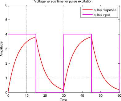
The Simulink model to investigate the pulsed response of series RC circuit consisting of pulse generator block, transfer function block and scope is depicted in Fig.15. The input and output waveform are both visualized on the scope.

input

R*C.s+1

Goto

From

Scope

Step

Transfer Fcn

An alternative Simulink model created for solving differential equations (22) along with transfer block is shown in Fig.16. In this model, there is a provision to select step or ramp excitation.

Simulink block diagram for series RC circuit

• 5.3    Simulation Model Using State Space, Approach III

Complex electric circuit can be alternatively solved using the system state equation and output equation. Mathematically, the state of the system is described by a set of first order differential equation in terms of state variables [28].

dx

— = Ax + Bu dt

y = Cx + Du                        (24)

The equation (23) represents the state equation and (24) represents the output equation.

The variable x represents the state of the system, u is the system input, and y is the output, A is system dynamics matrix representing the coefficient of state variable, B is the matrix of input representing the coefficient of input in state equation, C is the matrix of output representing the coefficient of state variable in the output equation, D is the direct exposure matrix input to output. The matrix A , B , C , D for RC series circuit can be obtained directly and is given as:

A =

C =

RC

- 1

B =

D =

RC

R

The Simulink model solution for (5) and (6) is depicted in Fig. 17. The model consists of step, ramp, manual switch, state space block and scope. In this model, one can select the input from ramp or impulse block using manual switch 1. There is a provision to select step input or ramp and impulse signal using manual switch.

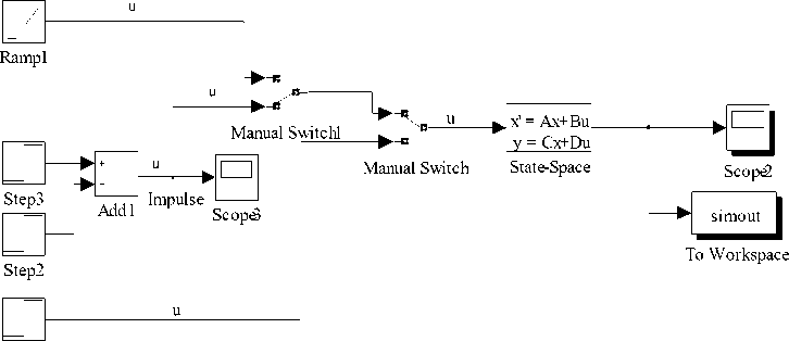
Step1

5.4 Modified Simulink Model using TransferFunction and State Space Together

The modified form of Simulink model using transfer function and state space approach is shown in Figure 18. In this model transfer function and state space block

both are used together. There is a provision to visualize system dynamics using step, ramp or impulse signal. Using multiport switch one can select the desired input. The selected input signal is applied simultaneously through state space and transfer function block using manual switch.

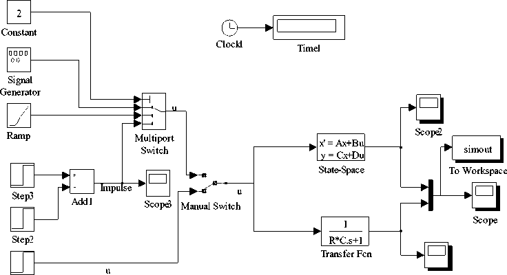
_Step1                                                                                        Scope4

• 5.5 Simulink Model Implementation Using User Defined Functions Library

• 5.5.1    Alternative Model Development Using Fcn Blocks, Approaches IV

• 5.5.2    Using S-function in Models

Alternatively, one can develop Simulink model of the series RC circuit using the Fcn Block of User-Defined Functions Library of Simulink packages. The Simulink flow diagram set up using the fcn block is shown in Fig. 19.

Simulink block diagram for series RC circuit

In this section, the Simulink model of (7) has been implemented using S function blocks of User Defined Functions Library. The S-function block is generally used to create customized or to add new general purpose block to Simulink or to build general purpose block that can be used several times in a model. Firstl of all, function m.file is developed and saved using name RC_ckt .m as depicted in Fig. 20.

MATLAB Solution function dx = RC_ckt (t,x,Vs)

%MATLAB function script: RC_ckt.m

% define model parameters

R = 2.5e3;

C = 0.002;

dx = -1/(R*C)*x+1/(R*C)*Vs end function[sys, x0, str, ts]=RC_ckt_sfcn(t, x, u, flag, xinit)

% RC_ckt_sfcn is the name of S-function

% This is the m-file S-function RC_ckt_scfn.m %

%M file S function implements a series RC circuit xinit = 0;

switch flag case 0 % initialization str = [];

ts = [0 0];

x0 = xinit;

% alternatively, the three lines above can be combined into a single line as

% [sys, x0, str, ts]=mdlinitializeSizes(t,x,u)

sizes = simsizes;

sizes.NumContStates = 1;

sizes.NumDiscStates = 0;

sizes.NumOutputs = 1;

sizes.NumInputs = 1;

sizes.DirFeedthrough = 0;

sizes.NumSampleTimes = 1;

sys = simsizes(sizes);

case 1 % Continuous state derivatives

Vs = u;

sys = RC_ckt(t,x,Vs);

case 3 % output sys = x;

case {2 4 9} % 2: Discrete state updates

% 3: calcTimesHit

% 9: termination sys = [];

otherwise error (['unhandled flag=', num2str (flag)]);

end

Fig. 20: MATLAB function script for analysis of RC circuit

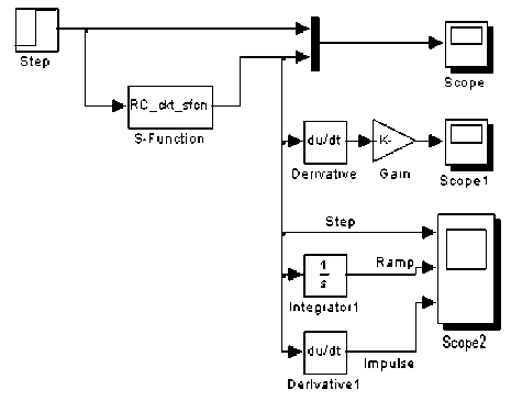
The Simulink model for S-function file is depicted in Figure 21. To incorporate an S-function into a Simulink model, the S function block from the User-Defined Functions Library is dragged into the model window. The name of the S-function is specified in the S-function name field of the S-functions blocks in dialog box.

waveform both are visualized on the scope. In the model, the impulse response is obtained by differentiating the step response, and ramp response is obtained by integrating the step signal.

• 5.5.3    Time Domain Model Development, Approaches V

The Simulink may be easily adopted in representing time domain response using various elements of Simulink block library. The corrosponding step, impulse and ramp response for the chosen design paramater is given as:

vc (t) = 10(1 - e -0.2 t)

Vc (t) = — e 5

t vc (t) = 10(t - 5(1 - e5))

The S-function name RC_ ckt_sfcn is defined in the block parameter dialog box. The model consists of step block, S function block and scope. The input and output

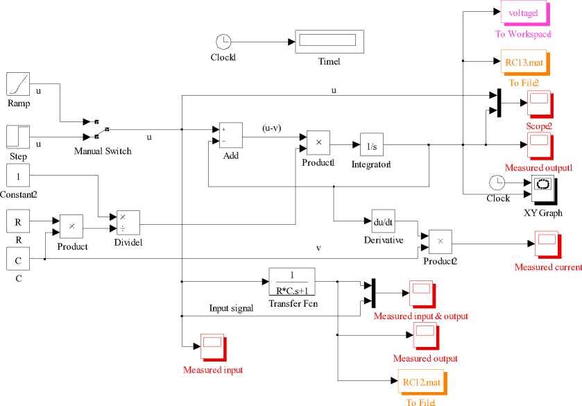
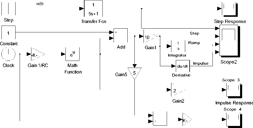
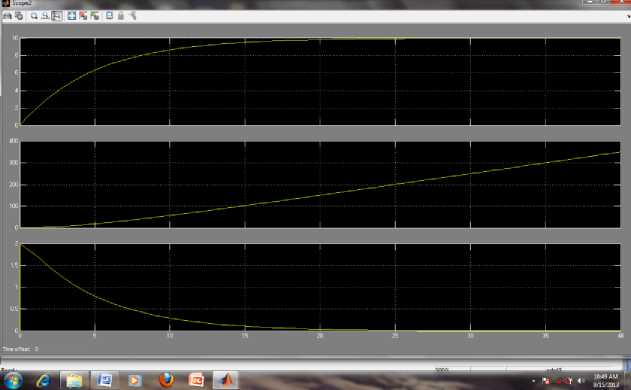
The system response of chosen circuit is also investigated by constructing a Simulink model using analytical time domain representation of (23), (24) and (25), and using TF approach as depicted in Fig. 22.

Response using frequency domain and time domain representation

Add1

Gain4

Ramp Response

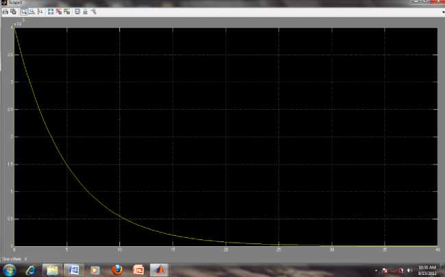
The Simulink model consists of clock blocks which generate time index vector, gain block, math function block, add block, integrator and derivative block. These blocks are dragged from the respective libraries, interconnected, and customized to set the model paramaters. The upper part of the model consists of step, transfer function and scope. The step response is obtained here using transfer function block and is depicted on the scope named Step Response. The lower part of the model consist of time domain implementation of step, impulse and ramp response and is displayed on scope 2,3,4 respectively. On block named scope 2, along with step response the ramp and impulse response is obtained using integration and derivatives blocks as depicted in the model. The impulse response is obtained by taking derivatives of step response, and the ramp response is obtained by integration of step response.

• VI. Data Driven Modeling

• 6.1    Directly From MATLAB Command Window

One can use Simulink together with MATLAB in order to specify data and parameters to the Simulink model. In data driven modeling, one can specify the system parameters commands in the MATLAB command window or as commands in an m.file in MATLAB script. The two cases are presented here:

In this approach, firstly the chosen system parameter variables are set in the functional parameters dialog box window for desired block of the model. The variable referred in functional parameters dialog window of the model are specified in the command window and simulation model is run from Simulink. An alternative Simulink model having the system parameters R, C specified in Simulink model transfer fcn block and U specified in step block functional parameter is depicted in Fig. 23.

Measured Current

The system variables defined in the command window are as follows:

>>R=2.5e3

>>C=0.002

>>U=10

• 6.2.1    MATLAB Script to Run the Simulink Model

• 6.2    Using m. file

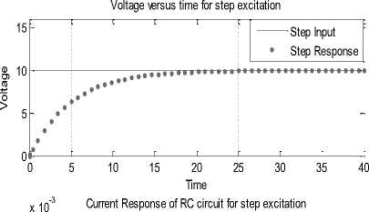
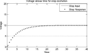
The MATLAB script used to call Simulink model of RCS10.mdl is shown in Fig.24. The MATLAB script RC_modelcall.m file defines system parameters, executes the simulation for given parameters, and plots the result. One can quickly change parameters of the model to simulate multiple cases through script file.

MATLAB Solution

% MATLAB script: RC_modelcall.m

R=2.5e3; %Resistance of the circuit in Ohms

C=0.002; %Capacitance of the circuit in Farads

U=10;      % Step input signal sim('RCS10') %run the simulink model 'modelcall.m'

% ********plot the simulation results**

subplot (2,2,1)

% plot simulation time index vector versus step input plot(ScopeData(:,1), ScopeData(:,2),'LineWidth',1) hold on

% plot simulation time index vector versus step response plot(ScopeData(:,1), ScopeData(:,3),'m.','LineWidth',1) xlabel('Time');

ylabel('Voltage');

title ('Voltage versus time for step excitation');

legend('Step Input','Step Response')

axis ([0 40 0 20])

grid on subplot(2,2,2)

% plot time index vector versus current response plot(ScopeData1(:,1), ScopeData1(:,2),'LineWidth',1) xlabel('Time');

ylabel('Current');

title ('Current Response of RC circuit for step excitation');

grid on % put grid on the axis subplot (2,2,3)

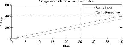
% plot simulation time index vector versus ramp input plot(ScopeData2(:,1), ScopeData2(:,2),'LineWidth',1) hold on

% plot simulation time index vector versus ramp response plot(ScopeData2(:,1),

ScopeData2(:,3),'m.','LineWidth',1)

xlabel('Time');

ylabel('Voltage');

title ('Voltage versus time for ramp excitation');

legend('ramp Input','ramp Response')

axis ([0 40 0 400])

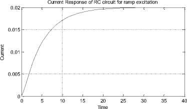
grid on subplot(2,2,4)

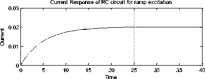
% plot time index vector versus ramp current response plot(ScopeData3(:,1), ScopeData3(:,2),'LineWidth',1)

xlabel('Time');

ylabel('Current');

title ('Current Response of RC circuit for ramp excitation');

grid on % put grid on the axis

Fig. 24: MATLAB script (RC_modelcall.m) used to call Simulink

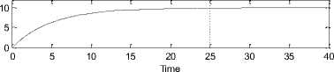
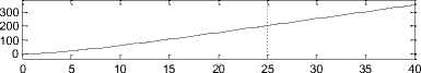
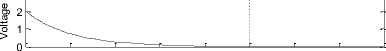
Results of system response to different inputs of various approaches using MATLAB simulation technique are presented in Fig. 25 to 35. The results of MATLAB script (RC1.m) using Laplace transform method symbolic simulation with step, ramp and impulse signals are presented in Fig.25.

Fig. 26 shows the simulation results of MATLAB symbolic simulation script RC2.m and plot of voltage versus time for step, ramp and impulse excitations using dsolve function. The symbolic simulation results are also presented using script RC3.m by changing system parameters. The results of simulations on executing the MATLAB script (RC3.m) are presented in Fig. 27, 28 and 29.

Voltage versus Time for step using LTM

0       5      10      15      20      25      30      35      40

Time

Voltage versus Time for ramp using LTM

Time

Voltage versus Time for impulse using LTM 3

0       5      10      15      20      25      30      35      40

Time

Fig. 25: Simulation result using symbolic simulation of (7) using LTM with step, ramp and impulse signal (RC1.m)

Voltage versus Time for step using dsolve

Voltage versus Time for ramp using dsolve

Time

Voltage versus Time for impulse using dsolve

0       5      10      15      20      25     30     35      40

Time

• V II. Results and Discussion

Fig.26: Simulation result using 'dsolve' function for analysis of RC circuit (RC2.m)

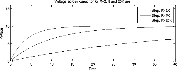
Fig. 27: Voltage across capacitor for different R using (RC3.m)

The voltage across resistor for R=2, 5 and 20 K Ohm, respectively is depicted in Figure 28.

Fig. 29 shows the current across resistor for different R=2, 5 and 20K Ohm respectively.

Fig. 27 shows the voltage across capacitor for R=2, 5 and 20 K Ohm respectively using step excitation. The variation in R implies the variation in time constant of the circuit. It is observed from Figure 27 that the larger is the time constant, slower is the response.

Current i(t) for R=2, 5 and 20K are

--•--Current, R=2K

Current, R=5K

Current, R=20K

J_______________________[_______ -------г-- ------------- Г_____.________ Г" " ________________[_______________ " Г

5                 10                 15                 20                 25                 30                 35                 40

Time

Fig. 29: Current across resistor for different R using (RC3.m)

It is observed that symbolic solution obtained using Laplace transform method of MATLAB script 'RC1.m' fully agrees with the plot generated using dsolve function of script 'RC2.m'.

Upon executing the MATLAB calling script (RC4.m), the result of MATLAB ODE script for analysis of RC circuit is presented in Fig. 30.

The running of script file (RC5.m) by typing the file name RC5 without having .m suffix in the command prompt, result into a solution that is graphically depicted in Fig. 31.

Step response

Voltage versus Time for step input using ode45

:                     | ^й Step response

Time

0       5      10      15      20     25     30      35      40

Time

Fig. 31: Simulation result using MATLAB ODE function handle using (RC5.m)

Fig. 30: Simulation result of MATLAB ODE script for analysis of RC circuit (RC4.m)

The execution of MATLAB code 'RC6.m' to evaluate the solution of RC circuit using transfer function for step, ramp and impulse excitation is shown in Fig.32.

Step response of series RC system

Time (seconds)

Impulse response of series RC system

0        5        10       15       20       25       30       35       40

Time (seconds)

Fig. 32: Simulation result of RC system using TF (RC6.m)

On executing the MATLAB script RC10.m, the results of MATLAB script are presented in Fig.35.

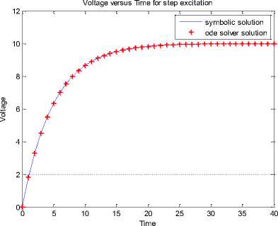
Fig. 35: Simulation result comparison of symbolic dsolve solution with a direct solution ODE solver (RC10.m)

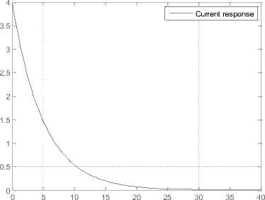
The execution of MATLAB script RC7.m results into the current response of RC system as presented in Fig. 33.

_{x 10}^-3               Current response of RC system

Time (seconds)

Fig. 33: Simulation result using script (RC7.m)

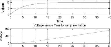
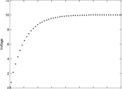
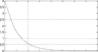
The execution of MATLAB script 'RC9.m' results into a solution in the form of a plot as presented in Fig. 34. The plot depicts capacitor voltage v ( t ) versus time for chosen parameters.

Voltage versus Time for step excitation

Time

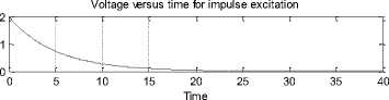
Fig. 34: Simulation result using time domain expression of (10), (13) and (16) respectively (RC9.m)

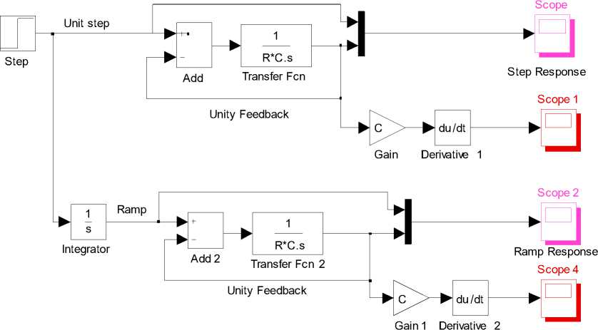
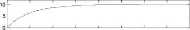
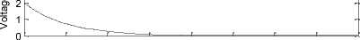
The system responses to different inputs using Simulink for first order RC circuit are presented in Figure 37-46, respectively. Fig. 37-38 presents the response of Simulink model (RCS1.mdl) for step and ramp excitations using differential equations for chosen system and simulation parameters. After running the model, one can visualize the output of Simulink model on the scope block by double clicking, or plot the result of simulation output by entering the plotting commands in command window or by writing script .m file. In this model, besides temporarily storing the simulation output in workspace, the result of simulation of model RCS1.mdl is also written to a MAT file named RC.mat, and RC1.mat using the 'To File' block. Fig. 37 depicts the voltage and current across capacitor for step excitation. Fig.38 shows the voltage and circuit current for ramp driving signal.

After the simulation is complete, one can also load the MAT file using script as shown in Fig.36.

% MATLAB script: RCMP1.m

%ScopeData contains the time, input and output vector subplot (2,1,1)

% plot simulation time index vector versus step input plot(ScopeData(:,1), ScopeData(:,2),'LineWidth',1) hold on

% plot simulation time index vector versus step response plot(ScopeData(:,1), ScopeData(:,3),'m.','LineWidth',1) xlabel('Time');

ylabel('Voltage');

title ('Voltage versus time for step excitation');

legend('Step Input','Step Response')

axis ([0 40 0 16])

grid on subplot(2,1,2)

% plot time index vector versus current response plot(voltage3(1,:),voltage3(2,:),'r.','LineWidth',1) xlabel('Time');

ylabel('Current');

title ('Current Response of RC circuit for step excitation');

axis ([0 40 0 4e-3])

grid on

Voltage versus time for step excitation

15      20      25

Time

4v

I

3^ •

1 Г                                                                               ’

0к------c------c------г ***••••••••••••••<••••••••••••■•

0       5      10      15      20      25      30      35      40

Time

Voltage versus time for ramp excitation

0^

t^tU***t*'

Ramp Input

Ramp Response

0       5      10      15      20      25      30      35      40

Time

0 -

Current Response of RC circuit for ramp excitation

^е»<=е№

0       5      10      15      20      25      30      35      40

Time

The input and output voltage across the capacitor using Transfer Function approach in Simulink model

On running the model RCS6.mdl, the results of simulation agree with earlier obtained results of Simulink model as created in section 5.1 to 5.3. The input, output voltage and current response for ramp excitation leading to result of simulation using Simulink model RCS7.mdl created using blocks of user defined function library is depicted in Fig. 42. The step response of the model fully agrees with the result obtained earlier.

The results of simulation of Simulink model

Time

[        impulse response

1.5

0.5

Time

The Simulink model RCS9.mdl and the model created in section 5.1, 5.2, 5.4 and 5.5 is being simulated using data driven modeling by defining the system paramaters as variables in the corrosponding blocks of Simulink model. The system paramater variable set in the paramater dialog box of Simulink model are either defined in the MATLAB command window or by calling the model using m.file with the system and simulation paramaters defined in the MATLAB script. The simulation results confirm with the result of Simulink model RCS1.mdl to RCS9.mdl. The Simulink model RCS10.mdl is also simulated by running MATLAB script RC_modelcall.m as depicted in Fig. 24. The results of simulation script are shown in the Fig. 46.

_{x 10}^-3       Current Response of RC circuit for step excitation

0       5      10      15      20     25      30     35      40

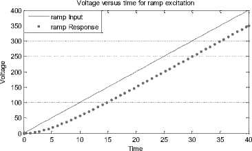
Fig. 46: Simulation results from MATLAB script file

Time

It is evident that same results are obtained by both specifying the parameters in command window and by running the model from MATLAB script.

It is observed that running the model with different apporches results into same corrosponding voltage/time, current/time plot for given input signal. It is evident upon inspection that all these methods produce the same result. Simulation and analysis of diverse engineering applications (first order RC circuit) based on differential equation, transfer function, state space representation, user defined function, time domain response using Simulink model is depicted in various suggested models as shown in section 5. The Simulink flow diagram of first order RC system shown in section 5 merely recreates the same simulation as using MATLAB script implementation depicted in section 4.

It is evident from these plots that the system response to various excitation conditions shows a similar output. In case of step signal, it is observed that smaller the time constant of the system, the faster is its response to a step input; or the larger is the time constant, slower is the response. At t = да the output of the system equals to step amplitude. In case of ramp response, as t = да the output of the system also becomes infinity and error signal becomes equals to time constant. The greater the time constant of the system, the greater is the error. In case of impulse signal, as t = да the output of the system decays to zero. The larger the time constant of the system, the greater will be the time required to bring the system output to zero.

The response of RC circuit using various approaches under different input conditions seems to be very similar and results are ideal under different excitations. The component value can easily be changed and the circuit can be re-simulated. In a similar manner, these approaches may be useful in deriving a solution for other diverse engineering applications by describing the behavior of various electrical, mechanical, biological, chemical or any other systems by the governing equations.

• V III. Scope of the work

The MATLAB script implementation and Simulink model presented in this study can be used in numerous diverse engineering applications. These equations occur in numerous settings ranging from mathematics itself to its applications to computing, electric circuit analysis, dynamics systems, biological fields etc. An approach similar to the one presented in this work can be used to model various engineering applications. Some of the applications for study may include:

• •    Biological process modeling

• •    Bacteria growth in a jar

• •    Tumour growth in body

• •    Insect population modeling

• •    Fish growth modeling

• •    Water discharge modeling from hole in a tank

• •    Radioactive decay of material

• •    Transient analysis of first order system

• •    Mass spring damper system

• •    Response analysis of series and parallel RLC circuit

• •    Automobile Suspension System

Second Order System Investigation

In general, many common systems are represented by a linear differential equation of 2nd order as follows:

d ² y ( t )           dy ( t )

,■   + 2 ^Z® « -— + to n y ⁽ t ) = to_n u ⁽ t )   (26)

d 2t          n dt      n          n where the variable y(t) and u(t) represents the output and input of the system, respectively. toH represents the natural frequency and ζ is the damping coefficient.

The transfer function of a general second order system is as follows:

H ( 5 ) = -^ = ---- ^to-----

X ( 5 )   5 ² + 2 to + to ;

where Y ( s ) and X ( s ) represent the Laplace transform of output and input and H ( s ) represents the transfer function of the system.

In the second order system investigation, three distinct cases are encountered for various values of damping ratio ζ. The different values of ζ decide the behaviour of the system. Any linear system can be studied under different values of damping ratio. This factor can have following three cases:

• 1.    ζ > 1, the roots of the characteristic equation are real and the system corresponds to over damped system.

• 2.    ζ< 1, the roots of the characteristic equation are complex conjugate and the system corresponds to under damped system. The time response is damped sinusoid.

• 3.    ζ= 1, the roots of the characteristic equation are real and repeated and the system represents critically damped system.

• 4.    ζ= 0, the roots of the characteristic equation are imaginary and the system provides oscillating output.

The various MATLAB and Simulink simulation approaches presented in section 4 and 5 can be applied to find the solution of various second order systems such as (26) and (27). With reference to second order system Simulink model using TF for three cases ^ = 1, 0 and 0.2, 0.4, 0.6 and ton = 1, is depicted in Fig. 47 and the result of simulation is shown in Fig. 48 and 49. In the same way, we can examine the effect of varying ^ for various second order systems, and system behavior can be re-simulated for all the three cases.

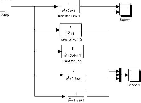
Transfer Fcn 4

Fig. 47: Simulink model of second order system using transfer function block given by (27)

applications as stated above. But, in a nutshell, the response of the first and second order systems can be achieved using the methodology presented here through MATLAB and Simulink. In fact, MATLAB presents several tools for modeling and simulation in circuit and system. These tools can be used to solve DEs arising in such models and to visualize the input and output relation. The work presented here can therefore be used in MATLAB Simulink based studies for a variety of applications.

IX Migrating from MATLAB to Open Source Packages

The work presented here can also be implemented using free and open source package Scilab and Xcos. Moreover, with some modification and moderate additional efforts, the solution of governing differential equation model developed in Simulink can be replaced by an equivalent free open source environment Scilab and Xcos [29].

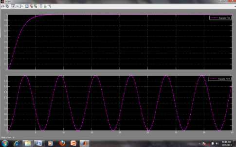
Fig. 48: Simulation result of second order system for ^ — 1,0 and

to n — 1 using (27)

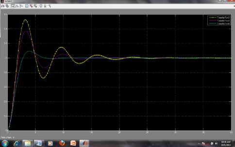
Fig. 49: Simulation result of second order system for ^ 0.2, 0.4 & 0.6 and to_n — 1 using (27)

X Conclusion

In the present study, first and second order system equations have been modeled, simulated and analyzed using different approaches involving MATLAB and Simulink. Moreover, through this communication, an attempt has also been made to demonstrate the usage of majority of blocks of Simulink sinks and continuous block library, and to present a brief idea about data driven modeling.

The methodology presented here using MATLAB and Simulink may serve as an inspiration for solving similar 1st and 2nd order ODE systems governing the behavior of diverse engineering systems such as those arising in many contexts including mathematics, physics, geometry, mechanics, astronomy, mechanical, civil, thermal, biological, population modeling and many others too. In fact, any continuous time system that can be modeled using differential equation, by transfer function, or the state variable can be simulated using MATLAB and Simulink. The process used here could very profitably be employed in the analysis of mechanical engineering course systems such as automobile, ship or air plane systems; and in chemical engineering courses in temperature control system, fluid level systems or in modelling of a chemical reactor.

Thus, in conclusion, it can be said that with model based design, it is feasible to bridge the gap between the theoretical foundation and practical applications, thereby cultivating innovation talents and promoting undergraduate level research. The work presented here prepares the students to accelerate innovation through simulation based engineering and sciences.

Due to the limitations of the length of the paper, it is not possible to cover other diverse engineering