Metadata based Classification Techniques for Knowledge Discovery from Facebook Multimedia Database

Published Online August 2021 in MECS

Social Media captures huge data that is shared by billions of people all over the world which leads too much difficulty to organize and arrange in a systematic manner. To set on this difficulty as well as to manage huge data, several Data Mining techniques have been developed such as Classification, association rule, clustering etc. In the present research work, Data Mining Classification techniques are used to label the Facebook data into respective classes [1]. Data can be mined using several Classifiers such as Bayes Classifiers, Rules Classifiers, Function Classifiers, Decision Tree Classifiers, Lazy Classifiers and more. These Classifiers contain several Classification algorithms. We have used Bayes Classifiers and Decision Tree Classifiers in this experiment to analyze the comparison between both as well as to test the discovered knowledge achieved by both the Classifiers [12]. The novelty of present experiment is to show which Data Mining algorithm works better in classifying Facebook social media data in an appropriate manner as well as with greater accuracy of Classification. To prove this, we had conducted literature survey of previous works proposed and found that, there were no such work has happened which can show, which Data Mining algorithm can classify the Facebook social media data with high accuracy. And to achieve that gap, in this experiment we are using eight different Data Mining algorithms to classify Facebook data.

Under Bayes Classifiers, we have considered four Classification algorithms that are, BayesNet, NaiveBayes, NaiveBayesMultinominalText and NaiveBayesUpdatable to calculate the Classification Accuracy of Meta Data ‘Type’. ‘Type’ is a Meta Data of Cosmetic Company’s facebook page dataset which contains four distinct attributes as status, link, photo and video. Our aim is to achieve the best Classification algorithm that can classify all four attributes in their respective classes with at most Accuracy [14].

Under Decision Tree classifiers, four Classification algorithms are used for calculating the Classification Accuracy of the same Meta Data ‘Type’ from the dataset. Those are J48, LMT, RandomForest, RandomTree [13].

The dataset is divided into two splits, training and testing. And to achieve this, percentage split method is used. It indicates that the part of the dataset is considered as training data and another part is considered as testing data. Using data mining Classification tool WEKA, we have calculated the Accuracy of correctly classified instances, kappa statistics, root mean squared error, relative absolute error, root relative squared error and generated Confusion Matrix which shows the different classes such as link, photo, status and video of type Meta Data. Classification error tables are generated for all 8 algorithms of two Classifiers. These tables show how many instances among total of 500 instances are correctly classified and also the number of incorrectly classified instances in tabular format.

As the dataset used in current work is, a company’s cosmetic product advertisement data hence, our is beneficial to those who wants to classify the social media data which is noisy and inappropriate all the time, the findings may help them by advising which Data Mining technique is better to classify the posts uploaded on the social media. By this, knowledge discovery can be achieved from enormous noisy data. The structure of the paper describes the proposed framework of the current work, dataset used in the research and its attributes then experimental results of Bayes Classifiers and results of Decision Tree Classifiers are described following with Classification error tables and also shown the comparison analysis of Bayes Classifiers and Decision Tree Classifiers based on different observations in the results produced by both the Classifier algorithms. Finally, concluded the content of the research experiment conducted.

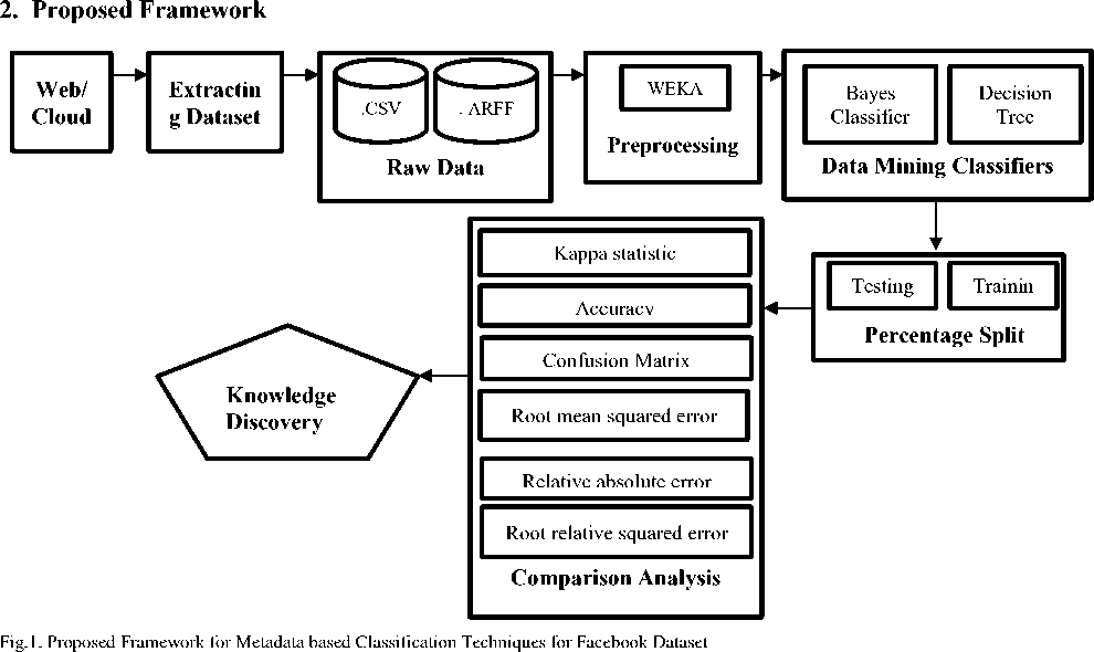
Fig 1 describes the framework of present work, how the experiment has been carried out. As mentioned in the abstract part, the cloud which is also determined as the web is full of data. In the initial step, the data is retrieved from the web. And the data is full of noise, inconsistency and several missing information which leads difficulty in arranging the data as well as to use for future predictions. Hence it is required to refine the raw data to use it efficiently. Retrieved data is stored in data storage either in .CSV stands for Comma Separate Value or in. ARFF form stands for Attribute Relation File Format. The raw data is preprocessed using WEKA preprocessor.

In the present experiment two Data Mining Classifiers are considered among several, those are Bayes Classifier and Decision Tree Classifier. Bayes Classifier has introduced several Classification algorithms and, in this work, we have used BayesNet, NaiveBayes, NaiveBayesMultinominalText and NaiveBayesUpdatable to calculate the Classification Accuracy of Meta Data ‘Type’. Under Decision Tree Classifier we have used J48, LMT, RandomForest and RandomTree algorithms.

In Classification technique, to check the accuracy and other findings of the data, the whole dataset should not be considered as either training or testing which leads in giving 100% Classifying accuracy for all the datasets when applied. So, it is necessary to partition the whole dataset in different parts. Methods like, percentage split, k folds cross validation test etc. are used to get the efficient Classification results. In present work, percentage split method is used which splits the dataset into two major parts as training data and testing data. The present work considers 66% of data as training data and remaining 34% as testing data.

Classification Accuracy, kappa statistics, root mean squared error, relative absolute error, root relative squared error have been formed for all the algorithms by calculating different estimates like TP value (True Positive), FP value (False Positive), Precision, Recall, F-Measure, MCC, ROC area, PRC area and Class. An efficient Confusion Matrix has been generated which labels the class for all the instances of Meta Data ‘Type’. Based on these results of all the algorithms, all calculated measures are compared, studied and analyzed in depth to make knowledge discovery by producing best Classifier of Facebook data that can label the data in appropriate classes and leads to knowledge discovery.

Page total	Type	Category	Post Mon1	Post Weel	Post Hour Paid	Lifetime P		Lifetime P
139441	Photo	2	12	4	3	0	2752	5091
139441	Status	2	12	3	10	0	10460	19057
139441	Photo	3	12	3	3	0	2413	4373
139441	Photo	2	12	2	10	1	50128	87991
139441	Photo	2	12	2	3	0	7244	13594
139441	Status	2	12	1	9	0	10472	20849
139441	Photo	3	12	1	3	1	11692	19479
139441	Photo	3	12	7	9	1	13720	24137
139441	Status	2	12	7	3	0	11844	22538
139441	Photo	3	12	6	10	0	4694	8668
139441	Status	2	12	5	10	0	21744	42334
139441	Photo	2	12	5	10	0	3112	5590
139441	Photo	2	12	5	10	0	2847	5133
139441	Photo	2	12	5	3	0	2549	4896
138414	Photo	2	12	4	5	1	22784	39941
138414	Status	2	12	3	10	0	10060	19680
138414	Photo	3	12	3	3	0	1722	2981

Fig.2. Dataset

The dataset has 19 different Meta Data and each carry 500 instances. Fig 2 shows a slice of the dataset used for current research.

• 2.1.    Percentage split method

• 3.    Data Mining Classifiers and Classification Algorithms

• 3.1.    Bayes Classifier

Percentage split method is used to partition the Facebook dataset used in present work. To calculate the Classification Accuracy of any Data Mining Classifier, the input dataset must be divided in two parts i.e., test data and training data, the first input dataset is fully considered as training data and to test that training data, we must provide a test dataset. These two datasets can be put into the Classifier and get some evaluation result separately then the Classifier makes predictions on first data from these two datasets [7]. Percentage split method is different from this method.

In Percentage split method, we use single dataset and divide the dataset into two parts. One part is used for training data and another is used for testing data. Perhaps two-third of the dataset is used for training and one-third of the dataset is utilized for testing. The important thing to be considered here is, the training data must be different from testing data [7]. If both are same, the evaluation results will mislead and they do not reflect the expected result in the form of new data when we apply it on any Classifier.

In the same way we have used single dataset in the present work and used Percentage split method to partition the dataset as training and testing. In our work, 66% of dataset is considered as training data and 34% dataset is utilized as test data. If we wish, we can consider different ratio also, for example, 60% for training and 40% for testing. In such cases we get slightly different evaluation results.

Two Classification methods are used to categorize the Facebook data those are, Bayes Classification method and Decision Tree Classification method. In this section eight Classifiers which belongs to above mentioned Classification methods are explained that we are going to use in further calculations of the present experiment.

Bayes Classifier works based on applying Bayes theorem [15]. The theorem works based on previous knowledge and describes the probability of an event. Mathematically Bayes theorem is formatted as,

Р(Л|В) ^М)^

v 1 J        P(B)

In the above formula, A and B are events.

P(B) ≠ 0

P(A|B) is conditional probability. Number of times event A occurring when B is true.

P(B|A) is also conditional probability. Number of times event B occurring when A is true.

P(A) and P(B) are marginal probability. Observing probabilities of A and B respectively [16].

• A.    BayesNet Classification Algorithm

BayesNet stands for Bayesian Network. It has V variables and E edges which forms G graph.

G = (V,E)

Edge E represent A i and A j

(A i , A j ) € E

Node represents the random variable

V = {A1,A2,A3   }

Random variable V holds the product of all conditional probabilities of A i for given P ai . The BayesNet represents it as,

Р(Л1,Л2,Лз..............ЛП) = П,-1НР(^)                              (2)

х * ШУ

• B.    NaiveBayes Classification Algorithm

NaiveBayes Classification technique can be determined as statistical predictor. The algorithm performs good at achieving class membership probabilities. It helps predicting the tuples belong to which respective classes hence it is also considered as multi class predictor. To calculate the posterior probability P(a|b) from P(a), P(b), P(b|a) the equation is,

У^У>)   ^('l)^'                                             (3)

Where P(a|b) represents the posterior probability of a class (a, target) for predictor (b, attributes)

P(a) represents earlier probability of class

P(b|a) represents the likelihood, probability of predictor given class

P(b) earlier probability of predictor

• C.    NaiveBayesMultinominalText Classification Algorithm

The algorithm performs only using string attributes. In the present work, Meta Data ‘Type’ is also of datatype string. It accepts other datatypes but ignores while classifying [17].

• D.    NaiveBayesUpdatable Classification Algorithm

• 3.2.    Decision Tree Classifier

The algorithm is an updated version of NaiveBayes Classification algorithm which is explained in the above section.

Decision Trees are constructed based on Greedy search method which classifies unknown records in quick manner. Decision trees handle continuous as well as discrete attributes and give clear Classification indications for predicting the classes. Decision Tree is supervised learning method and is developed for Classification and regression [2]. It plays a vital role in Knowledge Discovery and Data Mining because of its ability to handle missing values with huge data. The name suggests the structure of a Decision Tree is like forming a tree with root node, internal nodes following by leaf nodes [12,9]. In Fig 3. Structure of an example for Decision Tree is shown. The root class is Marks, Internal nodes are Fail, First Class and Second class, leaf nodes are FClass only and Distinction classes. Indicating the attributes in tree structure for Classification helps in clear understanding and analyzing [20,21].

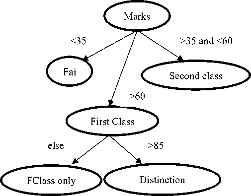
Fig.3. Example Decision Tree structure

• A.    J48 Decision Tree Algorithm

J48 Decision Tree is an advance version of C4.5. The algorithm applies divide-and-conquer rule while classifying the attributes of a dataset and uses measures like gain and entropy for calculations. To construct J48 Decision Tree [20, 21], pruning method is used. Pruning is a method of machine learning which is used to reduce the size of decision trees by clearing some sectors of the tree which seems not much useful for classifying the instances hence it helps in reducing the complexity of the tree [8, 9].

• B.    LMT Decision Tree Algorithm

Logistic Model Tree is supervised learning method. Used in Classification associated with logistic prediction. LMT Decision Tree uses linear regression method to build linear regression model and provides section wise classes to the instances of the dataset [10].

• C.    Random Forest Decision Tree Algorithm

Random Forest Tree works based on group learning method to conduct regression method, Classification and some other techniques which operate by constructing a multitude of decision trees during training period and producing the class that is the mode of mean prediction and classification of an individual tree. Random forests middling many profound decision trees, that are trained on numerous parts of the same training set for diminishing the variance [8].

• D.    Random Decision Tree Algorithm

• 4.    Results and Findings

4.1. Correctly classified instances

• 4.2.    Incorrectly classified instances

• 4.3.    Kappa statistics

  The technique, kappa was produced by “Jacob Cohen” in the journal Educational and Psychological Measurement in the year 1960. Kappa is a very good measure which can handle multi-class as well imbalanced class problems [4] in an efficient manner. The Kappa statistic works based on observed accuracy and expected accuracy. It compares an observed accuracy with expected accuracy . Here the term observed accuracy indicates the number of correctly classified instances in the Confusion Matrix. And the term expected accuracy is defined as the accuracy calculated by any random classifier based on the Confusion Matrix. The expected accuracy is directly related to the total number of instances of every class with the total number of instances classified by the Data Mining Classifier.

Random Decision Tree is a group learning method, generates decision trees randomly and conduct regression and Classification techniques. At each node of the tree, K random features are built by this and each node of the tree is split using the best split considering all instances to produce a standard decision tree. In case of a random forest, every node is split using the best among subset of predicators randomly selected at particular node. This is the way how random tree construction process is different from random forest [3].

Table 1 represents the calculated summary of correctly classified instances, incorrectly classified instances, kappa statistics generated by all the algorithms of both the Classifiers, Mean absolute error, Root mean squared error, Relative absolute error [19,20], Root relative squared error. All these mentioned attributes of Table 1 are explained below.

Table 1. Summary of Bayes and Decision Tree Classifiers

Name of the Classifier	Classification Algorithm	Correctly classified instances	Incorrectly classified instances	Kappa statistics	Mean absolute error	Root mean squared error	Relative absolute error	Root relative squared error
Bayes Classifier	BayesNet	129 75.88%	41 24.11%	0.3235	0.1319	0.3308	96.2373%	124.6664%
	NaiveBayes	91 53.52%	79 46.47%	0.2318	0.2322	0.4649	169.4273%	175.2081%
	NaiveBayesMultinominalText	143 84.11%	27 15.88%	0	0.137	0.2653	100%	100%
	NaiveBayesUpdatable	91 53.52%	79 46.47%	0.2318	0.2322	0.4649	169.4273%	175.2081%
Decision Tree Classifier	J48	156 91.76%	14 8.23%	0.6204	0.0604	0.1978	44.0817%	74.5644%
	LMT	154 90.58%	16 9.41%	0.6294	0.0467	0.2023	34.0796%	76.2536%
	Random Forest	159 93.52%	11 6.47%	0.7191	0.0659	0.1672	48.0583%	63.0035%
	Random Tree	148 87.05%	22 12.94%	0.4625	0.0647	0.2544	47.2206%	95.8746%

It shows the number of instances that are classified correctly in particular classes such as, status, link, photo and video. Table 1 is indicating the number of correctly classified instances form the testing dataset as well its percentage.

The number of instances that are classified incorrectly.

Cohen’s kappa is shown as:

_к _ Ро -Р е

1-Р е

= 1-

О)

In equation (4), K is the indication for Kappa. Po indicates observed accuracy and Pe indicates expected accuracy. According to standards, Kappa value is always less than or equal to 1. The kappa values 0 or less than 0 indicate that the Classifier is useless. That means it is not a standardized way for interpreting its values. According to Landis and Koch (1977) a kappa value < 0 indicates no accuracy in Classification, 0 – 0.20 gives slight Accuracy, 0.21 – 0.40 gives fair Accuracy, 0.41 – 0.60 provides moderate Accuracy, 0.61 – 0.80 gives substantial Accuracy, and 0.81–1 gives almost perfect Classification Accuracy [4].

• 4.4.    Mean absolute error

Absolute error is termed as the amount of error in the measurements. It shows the difference between the actual value and measured value. For example, if a scale shows our weight as 60kg but our actual weight is 59kg then the scale has an absolute error of 60kg – 59kg = 1kg. This is because of our scale is not measuring the correct amount we are measuring. For example, our scale might be correct to the nearest kilograms. If our weight is 59.5kg then the scale may consider the round up value and shows the weight as 60kg. In such cases the absolute error is 60kg – 59.5kg = 0.5kg. Now the mean absolute error is the average of all absolute errors found for all the instances of a dataset. In Data Mining, we can term it as in any test dataset, the mean of absolute values of each and every prediction error on all instances of test dataset is mean absolute error. Here the meaning of prediction value is the difference between true value and predicted value for that instance [5].

МЕА =

n^ i=i n |X i -X|

In equation 5, MAE is Mean Absolute Error. N represents the number of errors. ǀxi - xǀ represents the absolute errors. The equation conveys that, find all absolute errors and calculate the summation of them finally divide the value by the number of errors.

• 4.5.    Root mean squared error

• 4.6.    Relative absolute error

• 4.7.    Root relative squared error

• 4.8.    Total number of instances

• 5.    Confusion Matrix

It is the SD (Standard Deviation) of the prediction errors. Prediction errors are a measure shows how far from the regression line data points are. It shows how the data instance is concentrated around best fit line of regression.

RMSE = (VT-r^SI),                               (6)

In equation 6, RMSE represents Root mean squared error. SD y is standard deviation of Y. r is residual value.

Relative absolute error is, the mean absolute error divided by the corresponding error of the Classifier chosen for the dataset. Which means, the selected Classifier is predicting the previous probabilities of the different classes observed in the dataset.

Root relative squared error is, root mean squared error divided by the corresponding error of the Classifier chosen for the dataset. Means, the selected Classifier is predicting the previous probabilities of different classes observed in the dataset.

Shows the total number of instances present in the dataset used in present experiment i.e., 170 instances as testing data and remaining 330 instances as training data among total of 500 instances.

Is the summarization of predicted results from a Classification technique. Correctly and incorrectly predicted instances are described under particular class and the class along with its instances are arranged in matrix format, that is known as Confusion Matrix. It shows how the Classification technique is confused while predicting the instances under each class of the dataset. The result of the Confusion Matrix is totally depending on the Classification algorithm or the Classifier which we use for our dataset.

To calculate Confusion Matrix,

• ❖    Input: A valid dataset is required with expected outcomes

• ❖    Make prediction for every row of the dataset.

• ❖    Count the number of correct predictions and incorrect predictions from expected outcomes and predictions (see Fig 4 below).

• ❖    Organize these numbers in a matrix form.

Predicted Class

Actual

Class

	True	False
True	TP	FN
False	FP	TN

Fig.4. Construction of Confusion Matrix

Each row of fig 4 correspond to an actual class and each column corresponds to a predicted class [6]. Actual values are described by True and False indications and predicted values are described as Positive and Negative indications. Based on this, all the instances of the dataset are filled into the matrix. TP, FP, FN and TN indicate True Positive, False Positive, False Negative and True Negative respectively. And finally, to calculate the Accuracy of the Classifier, recall and precision values must be calculated.

True Positive: Positive tuples that are labelled correctly by the Classifier.

True Negative: Negative tuples that are labelled correctly by the Classifier.

False Positive: Negative tuples that are labelled incorrectly as positive by the Classifier.

False Negative: Positive tuples that are labelled incorrectly as negative by the Classifier.

Recall: Number of correctly predicted classes out of all positive classes that must be possibly high

Recall = TP / (TP + FN)

Precision: Number of correctly predicted classes out of all positive classes which are actually positive

Precision = TP / (TP + FP)

Accuracy: Out of all classes, the number of classes predicted correctly and it must be possibly high. And Accuracy is indicated by F-Measure. It is complex to compare two different models with high precision and low recall or vice versa hence to compare both the terms, F-Measure helps to calculate precision and recall on the same time.

F-Measure = (2*Recall*Precision) / (Recall + Precision)

• 5.1.    Confusion Matrix for Bayes Classifiers

Table 2. Confusion Matrix BayesNet Classification

a	b	c	d	^ Classified as
117	3	4	19	| a = Photo
1	10	0	4	| b = Status
9	0	1	0	| c = Link
1	0	0	1	| d = Video

The Cosmetic Company’s facebook dataset used in the present experiment contains 500 instances. The dataset is divided in to two sets that are, training data and testing data hence in testing data, 170 instances are chosen randomly. 170 because the percentage given for testing data is 34% and remaining 66% i.e.330 instances come under training data. The Confusion Matrix shown in Table 2 considers 170 instances for the Classification. Here BayesNet Classification technique is used. And 170 instances are classified in different classes as photo, status, link and video. 129 instances out of 170 are classified correctly and remaining 41 instances are classified incorrectly and the Accuracy of correctly classified instances is 75.88% which is shown in Table 1. In column ‘a’ of table 2, the first element of the first row has 117 instances which are classified correctly as Photo. Under column ‘b’ the second element of second row is holding 10 instances that are classified correctly as Status. In column ‘c’ third element of third row has 1 instance which is correctly classified as Link. And in the last column i.e., under ‘d’ fourth element of fourth row is also containing 1 instance which is correctly classified as Video. Except the mentioned elements, remaining 41 elements which are placed under different columns are misclassified by BayesNet Classifier.

Table 3. Confusion Matrix NaiveBayes Classification

a	b	c	d	^ Classified as
69	4	62	8	| a = Photo
3	12	0	0	| b = Status
1	0	9	0	| c = Link
0	0	1	1	| d = Video

Table 3 shows the Confusion Matrix generated by NaiveBayes Classification method. The Confusion Matrix holds both correctly and incorrectly classified instances of testing data. Out of 170 instances, NaiveBayes Classifier has correctly classified 69 instances as photo which is indicated in column ‘a’. 12 instances as status which is indicating by column ‘b’. 9 instances as link that is denoted under column ‘c’ and 1 instance as video under column ‘d’. Hence the Classifier has classified 91 instances correctly and remaining 71 instances are classified incorrectly and the Accuracy of correctly classified instances is 53.52% as shown in table 1.

Table 4. Confusion Matrix NaiveBayesMultinominalText Classification

a	b	c	d	^ Classified as
143	0	0	0	| a = Photo
15	0	0	0	| b = Status
10	0	0	0	| c = Link
2	0	0	0	| d = Video

Table 4 carries 170 instances which are classified in four different classes classified by NaiveBayesMultinominalText Classification. After observing the Confusion Matrix in table 4, 143 instances from the test data are classified correctly as photo and remaining 27 instances are misclassified as class photo only. We can say that, the algorithm is able is categorize the data in a single class. And the accuracy of NaiveBayesMultinominalText Classification is 84.11 % which is highest Accuracy among all four Bayes Classification methods used in the present experiment and we can make this comparison analysis from table 1.

Table 5. Confusion Matrix NaiveBayesUpdatable Classification

a     b    c    d	^ Classified as
69   4    62   8 3     12    0    0 1      0     9     0 0      0      1      1	| a = Photo | b = Status | c = Link | d = Video

Table 5 holds 170 instances classified by NaiveBayesUpdatable Classification method. This method is the updated version of NaiveBayes Classification but if we observe table 5 and table 3 there is no difference in classifying the instances. Updated version as well as actual NavieBayes method are working same on the dataset used in the experiment. Hence the Classification Accuracy is also same i.e. 53.52% which is shown in table 1.

• 5.2.    Confusion Matrix for Decision Tree Classifiers

Table 6. Confusion Matrix J48 Decision Tree Classification

a     b    c    d	^ Classified as
143   0    0    0 5     10    0    0 7     0    3    0 2     0    0    0	| a = Photo | b = Status | c = Link | d = Video

Table 6 contains the Confusion Matrix and the instances are classified by J48 Decision Tree Classification method. The method has classified 170 instances in three different classes and under class video, no instances are categorized. 143 instances are correctly classified as photo in column ‘a’, under column ‘b’, 10 instances are correctly classified as status and under column ‘c’, 3 instances are correctly classified as link. As shown in table 1, Classification Accuracy of J48 Decision Tree is 91.76% i.e., 156 instances are classified correctly and 14 instances are incorrectly classified by the Decision Tree.

Table 7. Confusion Matrix LMT Decision Tree Classification

a	b	c	d	^ Classified as
138	1	2	2	| a = Photo
4	11	0	0	| b = Status
5	0	5	0	| c = Link
2	0	0	0	| d = Video

Table 7 indicates the Confusion Matrix for Logistic Model Tree i.e. LMT Decision Tree. The tree has correctly classified 138 instances as photo, 11 instances as status, 5 instances as class link but it has not categorized any instance under class video and the Classification Accuracy of J48 Decision Tree is 91.76% shown in table 1.

Table 8. Confusion Matrix Random Forest Decision Tree Classification

a     b    c     d	^ Classified as
143   0    0     0 3     12    0     0 6     0    4     0 2     0    0     0	| a = Photo | b = Status | c = Link | d = Video

Table 8 is the Confusion Matrix for Random Forest Decision Tree Classification method. And according to table 1, this Classification method has achieved the highest Accuracy rate i.e., 93.52% among all eight Classification algorithms from Bayes Classifiers and from Decision Tree Classifiers considered in this experiment. Out of 170 instances of test data, 143 instances are correctly classified as photo class, 12 instances are correctly classified as status class, 4 instances are correctly classified as link class but no instance is classified as video class by this tree.

Table 9. Confusion Matrix Random Decision Tree Classification

a     b    c     d	^ Classified as
138   0    3     2 6     8     0      1 6     2    2     0 2     0    0     0	| a = Photo | b = Status | c = Link | d = Video

Table 9 contains the Confusion Matrix of Random Decision Tree Classification technique. As shown in table 1, the Accuracy of Random Decision Tree is 87.05%. It has 148 correctly classified instances and remaining 22 instances are incorrectly classified. Out of 148 correctly classified instances, 138 instances are categorized as photo, 8 instances are categorized as status, 2 instances are categorized as link and no instance is categorized under video class.

• 6. Conclusion

After the construction of all eight algorithms, four each under both Bayes Classifiers and Decision Tree Classifiers, we have studied all the measures using mentioned formulae under all the Classification methods and analyzed in depth for discovering the knowledge by Classifying the instances in particular classes with maximum Classification Accuracy. All the findings about both the Classifiers are shown in table 1. Based on different measures like Accuracy, Kappa Statistics, Mean absolute error and remaining all, we conclude that, the Decision Tree Classifiers are best suitable Classification methods to classify the instances of Facebook dataset in an efficient and methodical manner. As all four mentioned algorithms of Decision Tree are having highest Accuracy compared to Bayes Classifier algorithms.