Method for processing the results of cavitation tests of TNA pumps in order to obtain an approximating function

One of the most critical and energy-intensive components of a liquid-propellant rocket engine is a turbopump unit (TPU), which is necessary to ensure a continuous supply of fuel components to the engine chamber at a given flow rate and pressure. The following requirements are imposed on TPU as a unit of a liquid-propellant rocket engine (LRE):

• –    ensuring operability and basic parameters for a given resource with the necessary possible pauses of a specified duration;

• –    ensuring the supply of fuel components with the required flow rate and pressure in all engine operating modes, with a high degree of reliability, with an acceptable efficiency of the entire unit and a minimum manufacturing cost;

• -    ensuring the minimum size and weight of the entire propulsion system (PS) due to the smallest overall dimensions and weight of the TPU itself.

During the operation of the TPU, a cavitation phenomenon may occur in the pump, which adversely affects the fulfillment of the above requirements. Cavitation is the process of bubble growth in a liquid due to the dynamic decrease in pressure to saturated vapor pressure, which occurs at a constant temperature [1]. This process is similar to boiling (bubble growth caused by an increase in the temperature of the liquid). During cavitation, the bubble itself in the liquid changes dynamically: first, growth occurs, then, if it is not subjected to increasing pressure, growth will first stop and the bubble will begin to compress. The bubble will then collapse and probably disappear due to the dissolution of the gases and the condensation of the vapor. The collapse occurs abruptly if the vapor bubbles, or cavities, contain a small amount of gas, and less abruptly if the content in them is significant. Thus, cavitation includes a number of phenomena from the cjnception of a bubble to its collapse [2]. The phenomenon itself leads to a decrease in the operating parameters of the pump, which may affect the operation of the liquid rocket engine as a whole. With a longer exposure, due to local increases in pressure due to the collapse of the bubbles, cavitation causes deformation of the pump impeller - the so-called cavitation erosion.

Due to the impact of cavitation, there is a question of taking this phenomenon into account when designing a TPU and developing a technique that allows simulating the cavitation flow during pump operation. Such techniques exist. For example, they are described in [3; 4]. There are also methods of computational fluid dynamics (CFD) that make it possible to numerically simulate the cavitation flow in various units (pump impeller, turbine propeller, hydraulic wing, various objects in a liquid) and using media with different viscosities and surface tensions, including cryogenic ones. These techniques are presented in [5–7].

From a technical point of view, the oxidizer and fuel pumps are designed to supply fuel components to the gas generators and the engine chamber supply manifold. The main working element of the pump is a closed-type impeller with a one-way inlet, less often a two-way inlet [8]. To improve the anti-cavitation qualities of the pump, an auger is installed at the inlet in front of the impeller. Typically, the impellers are cast from a high-strength aluminum alloy; the screws are made of steel.

In the manufacture of a TPU, pumps are subjected to a number of tests to experimentally determine the quantitative and qualitative characteristics of an object as a result of forces acting on it during its operation, among which is a test to determine cavitation breakdown. As in general mechanical engineering, for testing pumps of a TPU, the types of tests can be classified according to the organizational and legal basis, their content, composition, location and test objects [9]. According to this classification, tests of pumps to determine cavitation breakdown can be classified as acceptance tests by organizational and legal type, parametric tests - by content, cavitation tests - by composition and bench tests - at the venue.

In consequence of a number of assumptions in various cavitation models, theoretical and practical data have a certain discrepancy. This discrepancy must be taken into account for the specifics of the operation of the pump of the TPU, namely, high differential pressure with small dimensions of the impeller. The aim of the work is to develop a technique for approximating the data of the hydraulic flow of pumps of a TPU for further verification of the model obtained with test data for a pump with a different geometry. The development and improvement of new methods for numerical simulation of hydrodynamic processes leads to an increase in energy efficiency and efficiency of a TPU and a LRE as a whole.

Description of measuring instruments

Measuring instruments (MI) for these tests were chosen so that the measurement error of individual parameters in the test mode, determined by the accuracy class of the MI, did not exceed the specified values:

• –    for expenses ±1.5%;

• –    for pressure ±1.0%;

• –    for differential pressure ±1.5%;

• –    for water temperature ±1%.

All appliances must be located in the correct position to ensure their stability. The position of the observer himself in all his actions should not cause obstacles when recording readings [10].

Miss detection and elimination

Typically, test data is recorded as the dependence of the head along the Y-axis, expressed in meters or in J/kg, against the inlet pressure along the X-axis, expressed in Pa or kgf/cm2. To be able to com- pare cavitation test readings with similar readings of other pumps, as well as to determine the function, we will reduce the values to dimensionless coefficients. For the X axis, we will use the cavitation number σ [2] written in the following form:

₌ 2О_1П-Р_Г)

,

P^fnav where Pin is the pressure at the inlet in MPa; Pv is the pressure of saturated steam in MPa; p is the density of the liquid in kg/m3. For the Y axis, we will use the head coefficient Ψ. This coefficient is used in a sufficiently large number of works, for example, in articles [11–13]:

^ = 2* g * H 2 , (2)

v ₂ ²

where H is the total head of the pump in m; v 2 is the speed at the pump outlet in m/s ² .

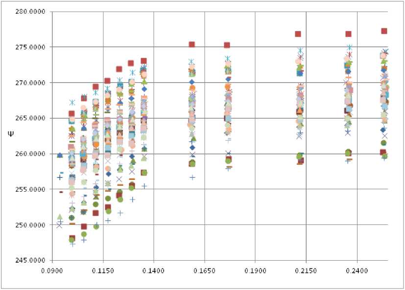
The results of the hydraulic tests with taking of the cavitation characteristics of a model (similar to a full-scale) pump with the obtained values of inlet pressure, outlet pressure, flow rate, impeller speed are entered in the table. For each test, readings are taken of the pressure parameters at the inlet and outlet of the pump, as well as the flow rate at 12–13 points. This article discusses the results of 78 virtual tests with a total number of 944 points, shown in Fig. 1. To determine the miss points, we use the Chauvenet criterion based on the Gaussian distribution. To do this, the number of standard deviations is determined, taking into account all the results, including potential misses, and then compared with the probability of a repetition of this event. The probability value is determined using a Gaussian distribution. To accurately determine the misses, let us divide all the points shown in Fig. 1 into groups from right to left over intervals of σ values: first group σ = [0,26–0,25], second [0,24–0,23], third [0,22–0,21], fourth [0,17–0,18], fifth [0,15–0,16], sixth [0,13–0,14], seventh [0,125–0,13], eigth [0,12–0,125], ninth [0,115–0,12], tenth [0,11–0,115], eleventh [0,104–0,11], twelfth [0,095–0,104], thirteenth [0,09–0,095]. There are 78 data points in each group, except for the 13th group, which has 8 data points. To work with the Chauvenet test, the mean and standard deviation values were calculated for each group. Let us consider the implementation of the Chauvenet criterion for all 13 groups.

In the first approximation, the lower points in groups from 12 to 5 did not fit the Chauvenet criterion (the value of the number of points of test values multiplied by the probability of repetition should not be lower than 0.5). We remove these points from consideration. Consequently, the number of points will decrease for these groups from 78 to 77, respectively. We recalculate the Chauvenet test for these groups.

According to the results of the second approximation, all points of groups 1–6 fit the Chauvenet criterion, while the lower points of groups 7–12 did not. We remove the test points from consideration again. In groups 7–12, the number of points will decrease from 77 to 76, respectively.

According to the results of the third approximation, the lower points of the 9th, 11th and 12th groups did not fit the Chauvenet criterion. Similarly, we remove these points from consideration. After this approximation, we can confirm that there are no gross misses in all groups, since the Chauvenet criterion is satisfied for all 12 groups.

Let us separately consider the points of the 13th group. There are no gross misses in this group, all 8 points are suitable for taking into account the tests. As a result of discarding misses, the total number of points to consider decreased from 944 to 927.

σ

Рис. 1. График данных испытаний

Fig. 1. Test Data Graph

Approximation of test results

To determine the function, its nature (linear, power, logarithmic, etc.), it is necessary to use one of the methods of mathematical analysis - approximation. To approximate the obtained results in order to obtain the dependence, we use the method of least squares [14]. The method consists in considering the sum of squared differences y i obtained during the cavitation test and the approximating function φ( x ) at the corresponding points. The function parameters a , b , c … n φ( x ) are selected so that the squared difference is the smallest. Depending on the type of function: a linear one of the form y = ax + b , a trinomial of the second degree y = ax ² + bx + c , etc., the systems of linear equations necessary to obtain the unknowns a , b , c differ.

When considering the behavior of the values of the pressure coefficient Ѱ on the cavitation number σ, which is common for all 78 tests, we can conclude that it is impossible to approximate the values with a linear dependence. As an approximating function, it is necessary to consider the logarithmic, exponential and power functions.

In the case of approximation by a logarithmic function, the dependence is given as F ( x ) = a + b * ln( x ). In the case of approximation by an exponential function, the dependence is given as F ( x ) = a * e^{b * x} . In the case of approximation by a power function, the dependence is given as F ( x ) = a * x^b . Using the method of least squares, we obtain the following approximation equations describing all 927 test value points:

F (x ) = 283.106 + 9.742*ln ( x);(3)

F (x) = 255.799* e(0'213* x);(4)

F (x ) = 283.78* x0-0369(5)

Based on the obtained equations, we will build a graph for each equation and compare them with the average values of groups 1–13 of the tests. The graph is shown in fig. 2.

The closest indications of the approximation and test values of the pump in the cavitation mode (the leftmost values of the points on the graphs) are shown by the power function (5). For further work on the approximation of the approximating function to the test readings, the exponential function will be taken as a basis.

To bring the values of the approximating function (5) closer to the graph of average test values, we set the coefficients for the function Ѱ: a = 0.35, b = –0.092456 and c = 1.0239. Let us write down the resulting approximating equation and compare it with the data of the average test values (Fig. 3):

a *0,0369                                     0,35*0,0369

a + Ь ,             (& - 0,092456) ,   ^,

T = 283,78 (     )----- = 283,78 (     ,        )------- .

c                      1,0239

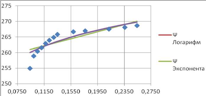
Рис. 2. График средних значений групп испытаний и их аппроксимации

Fig.2. Graph of average values of test groups and their approximations

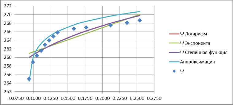
Рис. 3. График средних значений групп испытаний и сравнение с аппроксимирующем уравнением, логарифмической, экспоненциальной и степенной аппроксимацией

Fig. 3. Graph of average values of test group and comparison with fitted equation, logarithmic, exponential, and power fit

The maximum relative error of equation (6) and the average values of tests of groups 1–13 (Fig. 1) is 0.97%. However, if we compare equation (6) with the values of each test from the groups of points in Fig. 1 separately, then the maximum relative error will be 4.59%. For a more accurate approximation of the equation to the test data, let us consider the individual tests with minimum and maximum values of Ψ. Let us introduce new coefficients for equation (6) in order to understand the nature of the displacement of the approximating graph with respect to the values of Ψ. We will leave the exponent coefficient a equal to 0.35, and the coefficients for the values b will be taken equal to -0.094 and -0.0957, for the values c we will take equal to 0.998 and 1.07 for the minimum and maximum tests, respectively. Let us write down the obtained approximating functions:

T = 283,78

( a - 0.094 ) ^0,35 * ^0,0369

0.998

T = 283,78

( a - 0.0957 ) 0’ ³⁵ * ⁰ ’ ⁰³⁶⁹

1.07

To determine the approximating function common to all tests, which depends on the nominal value Ψ, we represent the dependence of Ψ on the coefficient in a linear form y = a * x + c . We obtain a system of equations for the coefficient b and c of functions (6), (7) and (8):

- 0,094 = a *277.2724 + c

- 0.0957 = a *259.4448 + c

'0.998 = a *277.2724 + c

• 1 .07 = a *259.4448 + c

  
  
  
  

We write the resulting approximating equation for the entire group of tests:

T = 283,78

a + ( T*0,000093577 - 0,

( - T*0,00403 8 + 2,11762 )

The formula (11) approximates the values of the function to the test data, except for the data that are in the test values close to the average. This difference becomes obvious if we consider the dependence of the coefficients b and c on Ψ. For an even more accurate approximation of the function (11) to the test data, we turn to the method of function interpolation using algebraic polynomials (polynomial interpolation). Let us use Newton's interpolation formula for unequal intervals [15]. This formula is a modified Lagrange formula and in general it can be written as follows:

f (x)= Bj +(x-Xj)B2 +(x-Xj)(x-x2)B3 +...+(x-Xj)*•••*(x-xn_JBn.

Using the divided differences, compiling an interpolation table, we find the coefficients B 1 , B 2 , B 3 … B n . For the coefficients of the difference b and division c , we obtain the equations:

a_diff = -0.094 + (6.27205 * 10“⁵) * ф„ - 277.2724) - (3.66748 * 10“⁶) * (T„ - 277.2724) * (T„ - 268.3439)

а^ = -0.998- 0.00290082 *(T„ -277.2724) -0.000127862 * (T„ - 277.2724) * (T„ - 268.3439)

Considering that in these eight tests there are 13 measurement points instead of 12, we change the coefficient –0.094 in formula (13) to the coefficient –0.092, the final formula for the difference coefficient b will be the following:

a_diff = -0.092 + (6.27205 * 10“⁵) * ф„ - 277.2724) - (3.66748 * 10“⁶) * (Т„ - 277.2724) * (Т„ - 268.3439)

Let us write the final test approximation function:

r        ^0SS*0 0S69

Т = 283,78^^                       (16)

adiv

The maximum relative error, when comparing the function (16) with each test schedule separately, does not exceed 1.9%. Preferably, the error is within 1% for most points. These values can be considered satisfactory.

Conclusion

During the analysis of the results, an overall good agreement between test data and function was found (16). The approximating function may have discrepancies at the beginning of cavitation tests; however, in the region of cavitation breakdown, it approaches the test values. When considering the relative error for all tests (excluding gross misses), the function shows the applicability to the test data. The additional coverage of the minimum and maximum test values gave more accurate approximations to the test data. In some comparisons, these functions and tests may differ more, which is explained by taking into account all test data, including those that have gone beyond the limits specified by the design documentation.

For further work, it is necessary to refine the coefficient b and c in order to increase the range of coverage of the values of σ and Ψ, as well as to increase the accuracy of the approximation. When considering the results of the approximation in terms of the possibility of applying function (16) to a similar approximation of the test values of other high-pressure pumps, it is necessary to clarify the coefficients a , b and c . The coefficients can be refined by applying them for the function (16) both as cavitation test data of other pumps (especially in this part, it is interesting to approximate the function to the test results of other high-pressure pumps typical for a TPU), and other methods of interpolation and approximation of coefficients and functions. Thus, the obtained method will make it possible to analyze the cavitation properties of a centrifugal pump in order to improve the anti-cavitation qualities of a TPU, thereby making it possible to meet modern energy efficiency requirements for new TPUs of a LRE being developed.