Method for unit self-diagnosis at system level

Published Online January 2019 in MECS

System level self-diagnosis was introduced by Preparata et al. [1] and since then it has been deeply investigated in a number of researches [2,3]. It aims at diagnosing systems composed of units, with the requirement that they are able to test each other by exchanging data through available links. At this level of diagnosis, each particular test is considered as atomic, which means that the details of test are abstracted (i.e., not considered), and only the result of test is taken into consideration.

As a rule, decision about the state of a system unit is made on the basis of the results of tests performed on it by other system units. In view of this, testing assignment and the number of testing units are very important for system diagnosis [4].

The decision about the state of a system unit can also be made on the basis of comparison of the outcomes produced by one unit with the outcomes produced by other units [5]. It is worth noting that comparing testing, as a self-diagnosis tool, was developed only for homogeneous systems. In case of comparing testing, a test is a comparison of the outputs between paired units performing the same task. Comparing the outputs from two units, it allows only to detect, but not to diagnose a failure. Comparing the outputs from more than two units, it allows to diagnose certain number of faulty units (resp. fault-free units) depending on the chosen diagnosis technique.

Recently, a comparison-based diagnostic model has been widely used in mobile ad-hoc networks [6,7] and swarm systems. Swarm systems can be found in nature and engineering areas. Examples of engineering swarm systems are systems such as unmanned vehicle formation systems, multi-robot systems, sensor networks [8,9]. A swarm system consists of nodes and the topology of nodes. The nodes are intelligent which means that they can process data by themselves. Nodes can communicate by exchanging of messages. Nodes of swarm system are prone to failure due to energy depletion and to their possible deployment in a harsh or hostile environment. Faults of nodes and faults related to the topology have significant influences on the operation of a swarm system and may have serious consequences. In view of this, the task of fault diagnosis is very important and still requires developing of more effective diagnosis methods and algorithms.

Generally, fault diagnosis in the swarm systems can be performed either by external diagnostor or by inner system resources. Although the external diagnostor can perform more effective fault detection by comparing to the system nodes, communication between the nodes and the external diagnostor can be problematic [5]. That is why much attention should be given to the fault detection based on the testing performed by system nodes (i.e., system self-diagnosis). Such self-diagnosis employs one of the following three architectures:   centralized, hierarchical and distributed architecture [8]. Centralized architecture uses one of the system nodes as an embedded diagnostor (or central node). Other nodes are not capable to perform diagnosis and they only send necessary messages to the diagnostor [10-12]. The main drawbacks of the centralized architecture are: strong dependence on reliability of embedded diagnostor; dependence on the state of communication between embedded diagnostor and system nodes; both communication load and computation load are increasing rapidly as the number of nodes increases. A hierarchical architecture was introduced in order to improve the scalability and reliability of the centralized fault diagnosis. In the given case, local diagnosis information is sent to the next layer of architecture for further diagnosis [13,14]. This architecture also depends considerably on reliability of system nodes. Apparently, a lesser is more extent than the centralized architecture. Distributed architecture was proposed to improve both centralized and hierarchical architectures. In this architecture, all nodes are equipped with fault diagnosis algorithm. Fault diagnosis for a node is achieved in a collaborative way and the results of the algorithms in the neighbors of the monitored node are all needed [15,16]. It is worth noting that distributed architecture is much more reliable than the centralized one and the hierarchical one. As a limitation of this architecture, we can consider the fact that each node may use incorrect information received from other nodes (i.e., this architecture depends considerably on reliability of information which a node receives from its neighbors).

System units can be subject to sophisticated attacks which attempt to manipulate the outputs of each unit [17]. In case, when system units are deployed in a hash or hostile environment, probability of fault of each unit is generally expected to be high [5]. Therefore, related or multiple faults of units are very probable. At present, some problems of fault diagnosis in swarm systems still remain. First, this concerns the topologies that may fail or change dynamically and the heterogeneous units [8]. In this paper, we propose the new method of system selfdiagnosis which can cope with all these situations (i.e., related or multiple faults of system nodes, changing topology and heterogeneity of nodes). Our method utilizes the results of series of tests performed by a node on other system nodes. The proposed self- diagnosis can deal with arbitrary topology (in the given case, it is called testing environment) and can be applied to heterogeneous systems in which a system node cannot be diagnosed by other system nodes. The proposed self-diagnosis can also cope with detecting and identifying the intermittent faults of nodes. An intermittent fault is a fault that produces negative effect only part of the time.

The key idea of this self-diagnosis consists in forcing the faults of a node to exhibit themselves during the testing which a node performs on other nodes. Particularly, the node faults could influence the results of tests. For each particular type of swarm system (e.g., multi-robot systems, sensor networks) evaluation of such influence can be done on the basis of results of special research. However, this task is beyond the scope of this paper. In the paper, we assume that a fault of a system node has effected the test results, and this fact is used for the fault detection. We also assume that each system node has a fault-tolerant part which always allows it to diagnose itself correctly. Similar assumption is made for self-testing of multiprocessors [18]. For the implementation of the method, it needs that a unit is capable to perform tests on its neighbors. The simulation performed on the basis of the proposed method enable evaluating the performance of the developed diagnosis algorithm and showing the efficiency of the suggested approach in the situations when majority of other approaches yield unsatisfactory results (e.g., in the situations when more than half of the system units are faulty).

The proposed diagnosis procedure is time consuming. In view of this, the paper focuses on the issue of determining the time needed for correct diagnosis. Particularly, we have determined how many times a unit must test the other system units in order to achieve highly credible result of diagnosis. The proposed selfdiagnosis was first introduced in previous research work [19]. In this paper, we have modified and improved the diagnosis of intermittent faults and performed complete modeling of unit’s self-diagnosis.

In the following sections, it will describe related works on the given topic in section 2. It will describe a proposed unit’s self-diagnosis for different faulty assumptions section 3. The developed diagnosis algorithm is presented in section 4. The results of the performed computer simulation are shown in Section 5.

• II.    Related Work

Comparison-based system level diagnosis has been researched in many papers, and it has been analyzed and structured in many surveys. This diagnosis was considered for possible implementation in wireless sensor networks, in multi-robot systems, in many-core processors and other areas.

In case of wireless sensor networks, researchers take into account the network topology (changed or fixed), types of possible node and communication faults (permanent or transient/soft/intermittent), protocol of communication among the nodes (one-to-one, one-to-many, one-to-all). Also, different comparing-based models were proposed (e.g., generalized, broadcast, probabilistic).

Application of comparison-based model in sensor networks allows a sensor node to identify its own status based on the information received from the neighbors [17, 20-22]. Alternatively, node state can be determined by the other system nodes [23, 24]. In case of multiple or related faults of sensor nodes, the unit diagnosis may be incorrect.

The developed comprehensive mutual diagnosis [25] is built on top of self- tests and presents a combination of self-testing and comparing approach. This diagnosis applied to multi-core arrays implies that each core first executes itself tests and generates a test signature. Then, it sends this signature to its four neighbors. Each core compares its own signature with those received from its neighbors. Comparing of signatures allows the core to detect faulty neighbors. The proposed in [25] mutual diagnosis also depends considerably on the state of the unit neighbors. The majority of comparison-based models impose an upper bound on the number of faulty units in the system. Some researchers consider faulty situations in which multiple and/ or related faults take place. Related faults or common faults consist of some system units simultaneously become faulty due to the same reason. J. Xu in [26] proposed to combine comparison testing with t/(n-1) - variant programming. It is worth noting that the adjudicator (i.e., diagnostor) in this scheme intends to detect only the correct variant. However, in practice it is also important to detect the faulty units (variants). In [27], the adjudicator with extended functionality was presented. This adjudicator allows to detect not only the correct units but also all the faulty ones. Both these papers consider independent and related faults. It is worth noting that these schemes were designed only for software systems to provide their fault-tolerance.

Mostly, the self-diagnosis performed on the basis of comparison-based model is used to detect permanently faulty system units [28, 22]. S. Chessa and P. Santi [24] have considered the problem of fault identification in ad-hoc networks and presented a comparison-based diagnostic model based on the   one-to-many communication paradigm. In this paper, the authors showed how both hard and soft faults can be detected. M. Elhadef et al. [6] have presented distributed comparisonbased self-diagnosis protocol for wireless ad hoc networks. The proposed protocol identifies hard and soft faults. P.M. Khilar  [29] proposed a distributed fault diagnosis algorithm for wireless sensor networks to diagnose intermittently faulty sensor nodes. It is worth noting that these researches do not consider a model to describe the behavior of soft/intermittent faults. However, the different behavior of such faults can have different impact on the system. A more detailed consideration of system faults which are different from hard faults will allow to provide a more effective system recovery.

Using the Bayesian approach for system diagnosis is a common practice. B. Krishnamahari and S. Iyengar [30] presented Bayesian fault recognition algorithm to solve the fault-event disambignation problem in sensor networks. X. Luo et al. [31] have proposed a fault-tolerant energy-efficient event detection paradigm for wireless sensor networks and presented Bayesian detection method.

In our paper, we also use this well-known approach to diagnose the state of a system unit. However, in this case, the event that a fault unit is split into three events. Explanation of such splitting is given in Section 5.

• III.    Basics of unit`s Self-Diagnosis

Normally, system level self-diagnosis provides unit diagnosis on the basis of the results of tests performed on the diagnosed unit. In view of this, the number of fault-free testing units and, consequently, the system testing assignment are very important for correct unit diagnosis [4].

In contrast, we propose to deal with the results of tests which a unit performs on other system units. It is expected that test results produced by a fault-free unit will be different from those produced by a faulty unit. Quality of such diagnosis depends considerably on the number of tested units, on the number of tests performed on each tested unit and also on the states of tested units.

For elucidation of the main parts of the proposed selfdiagnosis, we consider a simple example (Fig.1) with only one tested unit. It is assumed that unit u i has performed m identical successive tests on unit u j . It is also assumed that the states of testing and tested units do not change while all m tests are performed. We consider that each test result r_i j can take the value either 0 or 1, which depends on the states of tested and testing units and on the assumptions made in relation to the test results.

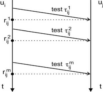
Fig.1. Repeated testing of unit u j .

Assumptions made about test results and their probabilities can be expressed with the help of Fig.2.

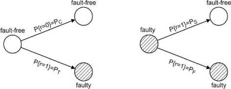
Fig.2. Test results and their probabilities.

In Fig.2, the following denotations are used:

P C is the probability that a fault-free unit will correctly diagnose a tested fault-free unit. This probability takes into consideration the fact that connection between units can fail;

P_T is the probability that a fault-free unit will correctly diagnose a tested faulty unit. This probability reflects the quality of test (e.g., fault coverage);

P_S is the probability that a faulty unit will produce the test result equal to 1 when a tested unit is fault-free;

P F is the probability that a faulty unit will produce the test result equal to 1 when a tested unit is faulty.

The assumptions made about test results can be specified and quantified. For example, PMC model [1] considers the following assumptions:

• •    Only permanent fault of a unit is possible;

• •    A fault-free unit always detects a fault in a tested unit (i.e., 100% fault coverage);

• •    Result of the test performed by a faulty unit is unpredictable not depending on the states of tested

units and can take the values either 0 or 1 with equal probability.

When the assumptions of PMC model are taken into consideration, the following specifications of the probabilities are possible: P C = 1, P T = 1 and P S = P F = 0 . 5. If the assumptions made in PMC model are applied to the test results in the considered example, then only two different tuples are possible (under the condition that unit u i is fault-free). Each tuple has the length of m and consists of the results of single tests.

The first tuple T 0 = (0 , 0 , .., 0) will be obtained when tested unit is fault-free, whereas the second one T 1 = (1 , 1 , .., 1) will be obtained when tested unit is faulty. When unit u_i is faulty, the tuple will be obtained, with great probability, contain both 0 and 1. It is followed by the assumptions which made about test results. Thus, diagnosis algorithm consists in the following. If the obtained tuple is either T 0 or T 1 , then the testing unit is fault-free. Otherwise, the testing unit is faulty. It is worth noting that faulty unit can also produce tuple equal to either T ₀ or T ₁. Probability of such result, P f _n , which can be determined as

P fn = P T 0 + P T 1                   (1)

where P_{T 0} is the probability of obtaining tuple T ₀, P_{T 1} is the probability of obtaining tuple T 1 .

If it assumes that all units have the same probability of fault, q , then

P t о = ( 1 - q )( 1 - P s ) m + q ( 1 - P f ) m

P_T i = ( 1 - q ) P + qP F ;

P fn = ( 1 - q )( 1 - P s ) m + q ( 1 - P f ) m +

+ ( 1 - q ) P sm + qP F .

Probability P f _n reflects Type II errors, and can be used for evaluating credibility of the performed diagnosis, D .

' D = 1 - P fn .                     (5)

Fig. 3 and Fig. 4 give the idea of how parameters m , q , P_S and P_F can influence the credibility of diagnosis result.

The proposed diagnosis will slightly change if some of the assumptions made about test results are different from those that are accepted in PMC model. For example, we can accept the assumptions of BGM model [32] according to which a faulty testing unit will always produce the result equal to 1 when it tests any faulty unit (i.e., P F = 1). Thus, one tested unit is used.

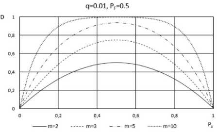
Fig.3. Functional dependence D = f (PS).

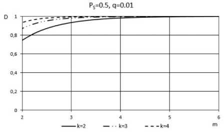
Fig.4. Functional dependence D = f ( m ).

Thus, the proposed diagnosis becomes less effective when only one tested unit is used. The effectiveness of the proposed diagnosis can be raised by using several tested units (Fig.5).

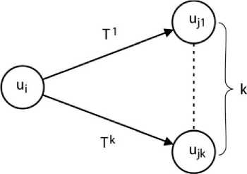
Fig.5. Repeated testing of k units.

When k tested units are used, we can expect, with great probability, that at least one of the tested units will be fault-free. This probability is equal to 1 - q ^k . Since a faulty testing unit after testing a fault free unit, it will get great probability (denoted as P_E ), and produce the tuple different from T ₁ and T ₀, we can use this fact as the basis for diagnosis algorithm. Probability P_E can be computed as

P e = 1 - P m - ( 1 - P s ) m            (6)

If testing unit is fault-free, all of the obtained tuples will be equal to either T ₀ or T ₁, which depends on the states of tested units. Thus, diagnosis algorithm is as follows. If each of the obtained tuples is either T 0 or T 1 , then testing unit is fault-free. Otherwise, testing unit is faulty.

Credibility of such diagnosis can be evaluated on the basis of probability P_E . Diagnosis will be incorrect if testing unit is faulty and event A_i , i ∈ [0 , 1 , .., k ] takes place. Here A i is the event when i tested units are fault-free, and each of the tuples is either of type T 0 or T 1 . Probability of event A i is determined as

P ( A i ) = C ^ q k " ' ( 1 - q ^P             (7)

where probability P_d = 1 - P_E .

Probability of incorrect diagnosis, P_ID is equal to:

k d = 1 - Pid = 1 -2 ckqk -i( 1-q Л =0

Thus,

Pid = E>( A i >  =£№ * - i ( 1 - q ) P d "      ⁽⁹⁾

i = 0              i = 0

It is worth noting that the probability of incorrect diagnosis, P_ID is computed under the condition that testing unit is faulty. Fig.6 and Fig.7 shows the idea of how parameters m , q , k and P S influence the credibility of proposed diagnosis.

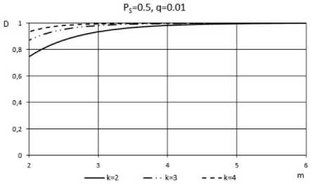
Fig.6. Functional dependence D = f ( m ) for the best case.

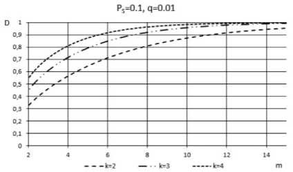
Fig.7. Functional dependence D = f (m) for the case of PS = 0.1.

Fig.6 presents the results for the case of P_S = 0 . 5. In the given case, credibility of diagnosis is greater than the credibility obtained for P S ≠ 0.5. Fig.7 depicts the credibility of diagnosis for P S = 0 . 1. Even for this worse case, the number of test repetitions doesn’t exceed a few dozens. For example, for k >  2, it is sufficient to repeat the tests 14 times to obtain highly credible result of diagnosis.

• IV.    Diagnosis of Intermittent Fault

Intermittent faults can be defined as the faults whose presence is bounded in time. More precisely, a unit can possess an intermittent fault but the effect of this fault is present only part of time. The amount of time of diagnosis procedure, t_d is important for diagnosis of intermittent faults. Depending on the amount of time t_d and on its position on the time axis (Fig. 8), the same fault may be identified as a permanent fault (case of t d¹ ) and as an intermittent fault (case of t d² ). There is also probability that the effect of intermittent fault will not be present during diagnosis procedure (case of t_d ³ ).

effect of IF is present effect of IF is present

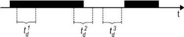
Fig.8. Diagnosis procedure and effect of intermittent fault.

Many researches have been done on the problem of diagnosis of intermittent faults. For instance, in [33], S. Kamal and V. Page considered the problem of the required number of test repetitions before a decision about the state of a digital circuit is made. At the beginning of testing, unit’s state is indefinite. Testing procedure (i.e., repetition of tests) is terminated either when a fault is detected, or on the basis of a decision rule. The authors suggested several decision rules for termination of testing procedure with the outcome indicating unit’s fault-free state. According to their research, the presence of intermittent fault in a unit can affect its behavior only part of the time. However, if the effect of an intermittent fault occurs during testing procedure, then such fault will be detected. Therefore, they described the behavior of intermittent faults (particularly, the occurrence of their effects) with the help of probability P ( S_i/w_i ), where S_i denotes the state of the unit when it possesses intermittent fault w i and the effect of the fault occurs.

Another approach to describe behavior of intermittent faults is presented in [34]. In this case, an intermittent fault has two states active (AS) and passive (PS). When an intermittent fault is in AS, the effect of intermittent fault is present. Whereas when an intermittent fault is in PS, its effect is not present. Transfers from one state to the other one are described with the corresponding intensities λ and µ (Fig.9).

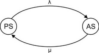
Fig.9. Model of intermittent fault.

where R is a set of all test results (so-called, syndrome), H ₁ is the hypothesis that a unit is fault-free, H ₂ is the hypothesis that a unit is faulty.

The prior probabilities of the examined hypotheses can be determined as P ( H 1 ) = ξ and P ( H 2 ) = 1 - ξ , where ξ is the probability that a unit is fault- free.

Decision about unit’s state can be made by using likelihood ratio

The process of transfers between these two states can be described as continuous Markov chain, where the time of the process being in the given state is random value. This random value has exponential probability distribution. In our research, we have adopted this model of intermittent fault because it enables us to model and to examine a wide range of intermittent faults.

It is assumed that if a testing unit possesses an intermittent fault which testing is in the AS at the moment, then the result of the test will be affected by this fault, and such intermittent fault can be detected. In the sequel, this fault can be identified on the basis of the affected test result(s). It is evident that it is possible to detect different types of intermittent faults depending on the time allocated to testing procedure. Here, we introduce two classes of intermittent faults.

To the first class C 1 , it refers to the intermittent faults which can frequently (more than once) appear in AS during testing procedure. To the second class C ₂, we refer the intermittent faults which can rarely (not more than once) appear in AS during testing procedure. The introduced classification of intermittent faults is relative and depends considerably on the parameters of testing procedure. Such classification of intermittent faults is important for diagnosis based on limited time of testing procedure.

P ( H 1 / R ) P ( H / R )

and a chosen threshold ω . The value of ω can be set on the basis of Bayesian discriminant analysis, so as to minimize the average misjudgment cost [35].

Thus, if χ ≥ ω , then hypothesis H 1 is accepted. Otherwise, additional measures should be undertaken to provide correct diagnosis.

The event that a fault unit can be split into three events P , C ₁ and C ₂, where

P is the event that a unit is permanently faulty;

C is the event that a unit possesses an intermittent fault of class C ₁;

C is the event that a unit possesses an intermittent fault of class C 2 .

For convenience, we denote with A the event that a unit is fault free, which corresponds to hypothesis H 1 . With account of these events, the conditional probabilities P ( A | R ), P ( P | R ), P ( C ₁| R ) and P ( C ₂| R ) can be expressed as

P ( A / R ) =-------------- ^ P ( R/A)--------------

^ P ( R / A ) + P_pP ( R / P ) + PP ( R / C ) + PP( R /C,)

P ( P / R ) =______________ P P P ^{( R} / P )______________

^ P ( R / A ) + P_pP ( R / P ) + PP ( R /C,) + PP( R /C₂)

P ( H / R ) =

P ( H ) P ( R / H )

Z 2 = 1 ^P ( W ( R / H i ) ’

P ( c i / R ) =

P c P ( R / C 1 )

^ P ( R / A ) + P_pP ( R / P ) + PP ( R / C_x ) + P_CP ( R / C₂ )

• V.    Decision rule for Unit`s Self-Diagnosis

As a rule, diagnosis algorithm is executed when checking procedure detects an error in system. The proposed unit’s self-diagnosis adopts this approach, which means that if all test results are equal to 0, which suggests no diagnosis algorithms are executed. When at least one test result is equal to 1, diagnosis algorithm should figure out whether the unit is fault-free or not. This is done on the basis of the accepted decision rule.

We recommend using Bayes’ rule

P ( H i / R ) =

P ( H ) P ( R / H ) Z 2 = 1 P ( H i ) P ( R / H i )

P ( C, / R ) =

_____________ P c P ( R / C 2 ) _____________

^ P ( R / A ) + P_pP ( R / P ) + PP ( R / C_x ) + P_CP ( R / C, )

where ξ + P P + P C 1 + P C 2 = 1.

• •    P_P is the probability of the event that a unit is

permanently faulty;

• •    P_{C 1} is the probability of the event that a unit

possesses an intermittent fault of class C ₁.

• •    P_{C 2} is the probability of the event that a unit

possesses an intermittent fault of class C 2 .

Given P P , P C and P C , it is possible to compute conditional probabilities P ( A | R ), P ( P | R ), P ( C 1 | R ) and P ( C ₂| R ) and then it needs to choose two of them which have the greatest values.

• V I. Considerations Behind the Diagnosis Algorithm

The situation when only one test result is not equal to 0, it means that the total number of “1” in the obtained syndrome R is equal to 1. It denotes such syndrome as R 1 . This situation is possible only when performing test τ ij either testing or tested unit at the moment, or both of them possess an intermittent fault in active state. In view of this, for examining this situation we suggest the following three hypotheses:

• •    h 1 : unit u i possesses an intermittent fault in AS and unit u j is fault-free;

• •    h 2 : unit U j possesses an intermittent fault in AS and unit u_i is fault-free;

• •    h 3 : both units u i and U j possess an intermittent fault in AS.

The probability of hypothesis h 3 is much lesser than the probabilities of hypotheses h 1 and h 2 . In view of this, only hypotheses h 1 and h 2 are considered.

According to the Bayes’ rule

unit u_i is fault-free. When the obtained syndrome contains more than one test results not equal to zero, it is necessary to compute conditional probabilities of receiving particular syndrome when a unit possesses certain type of fault (permanent, intermittent of class 1 or intermittent of class 2). Accurate determination of these probabilities presented in [4] which requires additional information about intermittent faults. In practice, obtaining this information is very difficult.

In view of this, we suggest the approximate method. This method consists in using approximate assessment of these conditional probabilities. Particularly, we assess these probabilities as either “very high” or “very small”. In the latter case, we consider these probabilities equal to zero and omit them. This approach bears some resemblance to the techniques based on fuzzy logic [36, 37], as mentioned in [38] for an example.

Given P C , P T , P S and P F , each tuple T ^α , α ∈ [1 , .., k ] can be expressed with the help of the table containing the total number of “1” in the tuple. For P C = 1, P T = 1, P S = 0 . 5 and P F = 0 . 5 such table takes the following view.

and

P ( h i /( r j = 1 ) =

P ( h i ) P (( r j = 1 )/ h i )

£ P ( h ) P (( r j= 1 )/ h ) i - 1

Table 1. Total number of “1” in the tuple

Total number of “1” in the resulting tuple, s		Tested unit
		A	P	C 1	C 2
Testing unit	A	0	m	1 ≤ s < m	0 U 1
	P	Chi{m/2}	Chi{m/2}	Chi{m/2}	Chi{m/2}
	C 1	0 ≤ s < m	1 ≤ s < m	1 ≤ s	0 ≤ s < m
	C 2	0 U 1	( m -1) U m	1 ≤ s < m	-

P ( h 2 /( r = 1 )

P ( h 2 ) P (( r j = 1 )/ h 2 )

£ P ( h ) P (( r j = 1 )/ h ) i - 1

Consequently

P ( h /( r j = 1 )) ₌ P ( h 1 ) P (( r = 1 )/ h ) P ( h 2 /( r = 1 ))   P ( h 2 ) P (( r j = 1 )/ h 2 )'

If information about the current state of unit u j is not available, then P ( h 1 ) = P ( h 2 ). If we assume that a unit possessing an intermittent fault in AS can produce test result 0 or 1 with equal probability, then P (( r_i j = 1)| h ₁) = 0 . 5. In case when P_C = 1 and P_T = 1, probability P (( r_i j = 1)| h ₂) = 1. Thus,

P ( h 1 /( r j = 1 ))

P ( h 2 /( r j = 1 ))

In the table, the Chebyshev’s inequality for the case when mp = m/ 2 is denoted as Chi { m/ 2}.

When a fault-free unit tests a fault-free unit (suppose m times), the resulting tuple will contain the total number of “1” equal to zero (in the table, see the intersection of the first row and the first column). When a tested unit is permanently faulty, the resulting tuple will contain the total number of “1” which is equal to m . When a tested unit possesses an intermittent fault of class C 1 , the resulting tuple will contain “very high” probability, the total number of “1” satisfies the expression 1 ≤ s < m . If a tested unit possesses an intermittent fault of class C ₂, then the resulting tuple will contain, with “very high” probability, the total number of “1” is equal to either zero or one (in Table 1, it is denoted as 0 ∪ 1).

Results produced by a permanently faulty unit are similar to tossing of fair coin. When a permanently faulty unit can produce result either 0 or 1 with equal probability, the total number of “1” in m tests (considered as Bernoulli trials) will follow the Chebyshev’s inequality

If unit u j with certain probability η , it possesses an intermittent fault, then

К >   ^var( s )

p{|s - mp\ > s } <     ₂

P ( h 1 /( r j = 1 ))   1 - n

P =-----------=---

^P  P ( h 2 /( r j = 1 ))    2 n

•

where var ( s ) is the variance of s , i.e. var ( s ) = mp (1 - p ).

Let’s set the deviation of s from mp as three or more standard deviations, i.e.

The higher the value η is, the greater our confidence is.

е = 3 4mp ( 1 - p ). (22)

Thus, Chebyshev’s inequality will be formed as:

P {| s - mp >  3 4mp ( 1 — P ) } ^ ¹ . (23)

For example, for m =100, it gets:

• P {| 5 - 50| <  15 } > 8 . (24)

In other words, when the probability is greater than or is equal to 0.888, the total number of “1” in 100 tests performed by a permanently faulty unit will be in the range 35 < s <  65.

As distinct from permanently faulty units, a unit possessing an intermittent fault of class C 1 doesn’t have such consistent pattern in producing tests results as a permanently faulty unit can produce. This fact allows us to discriminate between permanent and intermittent faults. In the given case, achieving correct diagnosis is not very important. As a rule, incorrect diagnosis results in a permanently faulty unit is diagnosed as a unit with an intermittent fault whose behavior is very similar to a permanently faulty unit.

We assume that the probability that both testing and tested units possess an intermittent fault of class C 2 and both these intermittent faults are in AS during the same testing procedure is so small that it can be neglected. In the Table, this situation is depicted as “-”.

According to the above considerations, the sought conditional probabilities P ( R | A ), P ( R | P ), P ( R | C 1 ) and P ( R | C 2 ) can be determined approximately. More accurately these conditional probabilities can be determined by taking into account the fact that probability distribution of random variable s is not discrete uniform distribution.

Then, probabilities P ( A | R ), P ( P | R ), P ( C 1 | R ) and P ( C ₂| R ) can be determined by using expressions (12) to (15).

Having computed conditional probabilities P ( A | R ), P ( P | R ), P ( C 1 | R ) and P ( C 2 | R ), we can choose two most probable hypotheses and then compute the likelihood ratio χ .

In case when χ < ω , and testing procedure can be continued, we increase either m , or k , or both. After performing additional testing, the value of χ is computed anew.

• VII. Diagnosis Algorithm

The diagnosis algorithm summarizes and integrates all the results of the above considerations. The initial data for the algorithm are as follows:

• -    diagnosis model (i.e., assumptions about allowable faulty model, about the probabilities presented in Fig.2, about allowable classes of intermittent faults, about homogeneity of units, etc.);

• -    unit statistical characteristics (e.g., those related to reliability and intermittent fault behavior);

• -    requirements to credibility of diagnosis result;

• -    time available for diagnosis.

Flowchart of diagnosis procedure is shown in Fig.10. The value of m (i.e., the number of rounds of testing) can be set either on the basis of available time or on the basis of the results of simulation. For the given unit’s reliability and the given intermittent fault parameters, simulation allows to determine the value of m which ensures high credibility of diagnosis result.

When information about possible intermittent faults is absent, the worst case can be modeled. In the given case, the “worst” parameters of intermittent faults are used. Diagnosis of intermittent faults with such “worst” parameters requires high values of m . In this case, for calculating the value of χ these worst parameters of intermittent faults should be used.

When information about possible intermittent faults is present, the interested party can use the known parameters and can set the acceptable threshold ω by taking into account the possible risk.

They can also make decision on possible changes of diagnosis procedure (e.g., value of m ) which will allow to achieve better diagnosis results.

• V III. Computer Simulation

With the aim to verify the correctness of the diagnosis algorithm, the computer simulation was performed. The simulation involved the following tasks:

• •    simulation of changes of units’ states;

• •    simulation of testing procedure for obtaining syndrome;

• •    processing the obtained syndrome (i.e., performing diagnosis algorithm).

The first two tasks were solved by using Petri Nets, and the third one was fulfilled in the web application [14]. The main parts of this web application are shown in Fig.11.

In Fig.11, z-score means standardized value indicating the number of standard deviations above or below the mean. For the case under consideration, the mean is equal to m/ 2.

Petri Nets have proved as very efficient tool for providing modeling and simulation of tests performed by one unit on other ones [39]. We are going to elucidate the simulation performed by using Petri Net (PN) with a simple example. Assume that unit u 0 tests two other units, u 1 and u 2 , in round-robin manner. The Petri net that depicts the units’ states, tests and test results is shown in Fig.12.

Modeling of units’ states is depicted at the top of Fig.12. The figure presents the case when all units possess intermittent faults.

Unit with intermittent fault has two states, AS and PS, (Fig.9) which are modeled by places PAS and PPS, and by two timed transitions, Tλ and Tµ.

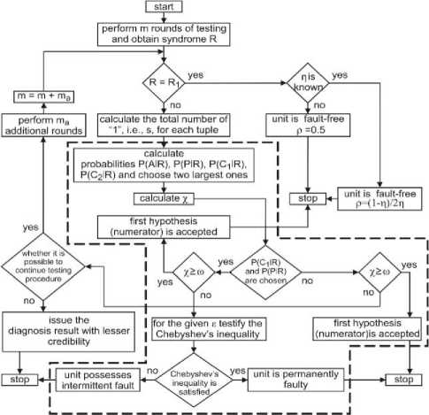
Fig.10. Flowchart of diagnosis procedure.

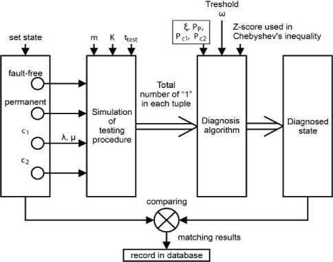
Fig.11. Main parts of application.

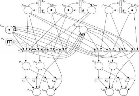
Fig.12. Petri Net used for simulation of testing procedure.

Duration of tests and the pairs of units which are involved in each test are modeled by timed transitions

T τ 11 , T τ 12 , T τ 13 , T τ 14 , T τ 21 , T τ 22 , T τ 23 , T τ 24 , and by places P_{τ 1}, P_{τ 2}, P_{τ 3}, P_{τ 4} (in the middle of Fig. 12). And finally, the test results are modeled with the help of immediate transitions t r 1 , t r 2 , t r 3 , t r 4 , t r 5 , t r 6 , t r 7 , t r 8 and by places P r 10 ,

P r 11 , P r 20 , P r 21 (at the bottom of Fig. 12). PN has also additional places P m , P test 1 and P test 2 . Place P m is used for simulation of m rounds of testing. Places P_{test 1} and P_{test 2} are used to model the order of tests execution. In the given case, unit u ₀ tests units u ₁ and u ₂ sequentially, not concurrently. The whole simulation procedure is presented on web site [40].

One of the main tasks of the simulation was to choose among the enabled transitions in each marking that transition actually fires. The choice is made on the basis of probability mass functions. Thus, we exploit the construct which is called a random switch [41].

At the beginning, the initial marking for the places that model unit’s states is determined. This is done on the bases of the units’ states which are set by researcher. When unit’s state is set as having an intermittent fault, the probabilities of AS and PS for the first initial marking will be computed according to the following expressions:

P PS = µ/ ( λ + µ ) and P AS = λ/ ( λ + µ ).

Then, by using random switches, the resulting marking is computed. In the resulting marking, we are interested in the places that model the test results (for the above example these places are P r 11 and P r 21 ).

The simulator clock is updated with the constant value equal to duration of test, t_test . The time needed for a testing unit to move the focus to the next unit for testing is very small and is neglected here. Every time after each clock update, new initial marking is determined only for the places modeling the unit states, and then the resulting marking is updated. As a result, the tokens are accumulated in the places which model test results.

For each updated initial marking, the probabilities P_PS and P_AS are determined as

P_AS = 1 - e ^{- λt} if the previous clock update at the end, the intermittent fault was in P_S .

P PS = 1 - e ^{- µt} if the previous clock update at the end, the intermittent fault was in AS , where t = t test .

In the resulting marking, the places that model test results will contain the total number of tokens equal to the total number of “1” in the tuples, and, thus, give the input data for the diagnosis algorithm.

Hence, algorithm for simulation of testing procedure can be outlined as follows:

begin for i:=1 to (m × k) do begin

• compute initial marking;

• initial marking -→ resulting marking;

end

• calculate the number of tokens in the places that model test results;

end

The main elements of diagnosis algorithm are shown in Fig.10 within the area bounded by dashed line. Diagnosis algorithm was written in PHP and is used by web application [40]. By exploiting this web application, a simulation of various faulty situations is performed to assess the quality of the developed diagnosis algorithm.

Fig.13 shows the probability of correct diagnosis, P_det .

During the simulation, the state of the testing unit was constantly set as permanent fault. For each execution of testing procedure, the state of each tested unit was arbitrarily set as either fault-free, or permanently faulty, or intermittently faulty ( C 1 or C 2 ). Results of simulation have shown that reliability of the tested units has minor impact on diagnosis result. On the average, twelve rounds are sufficient to obtain P_det greater than 0.99 regardless of what faulty sets are allowed, even when all of the system units are faulty. The required number of rounds, m , reduces to 8 if the number of faulty units (with permanent or intermittent faults) is lesser than ( k + 1) / 2.

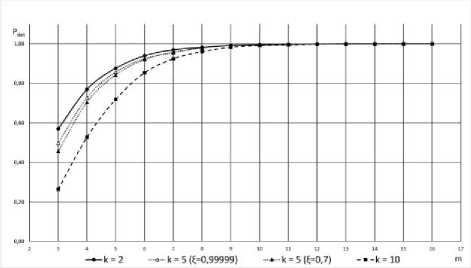
Fig.13. Probability of correct diagnosis of permanently faulty unit.

♦ - for the case when all the tested units are faulty

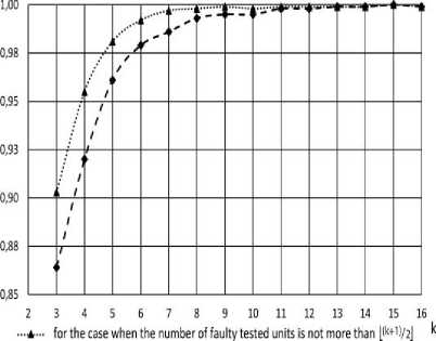
Fig.14. the probability of correct diagnosis of fault-free unit.

Fig.14 shows the probability of correct diagnosis. In the given case, incorrect diagnosis represents a Type I error (i.e., false positive). During the simulation, the state of the testing unit was constantly set as fault-free. The number of rounds and the reliability of tested units had a minor impact on diagnosis results. Fig. 14 depicts the case when m = 2 and ξ = 0 . 9999. If only faulty sets with not more than ( k + 1) / 2 arbitrarily faulty units are allowed, the probability P_det becomes greater than 0.99 when k ≥ 5.

Fig.15 depicts possible intermittent faults expressed via parameters λ and µ . Each intermittent fault is presented as a point with coordinates ( λ , µ ). A denotes the subset of intermittent faults that do not belong to class C 1 . B denotes the subset of intermittent faults that produce the effect similar to the effect produced by a permanent fault. We examined only intermittent faults that do not belong to subsets A and B . Basing on the simulation results, we have determined the subset of intermittent faults, denoted as C , in which every intermittent fault can be correctly diagnosed. Specifically, the probability of correct diagnosis of intermittent fault that belong to subset C is greater than 0.94 (for k = 4, m = 16 and z-score= 0.5).

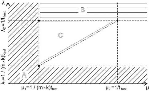
Fig.15. Subsets of intermittent faults.

The impact of z-score on the probability of correct diagnosis was investigated for intermittent faults belonging to subset C , and is shown in Fig.16.

It should be noted that the proposed method allows increasing the probability of correct diagnosis if statistical characteristics of possible intermittent faults are taken into account.

• IX. Conclusion

The paper presents a novel approach to system level self-diagnosis. Traditionally, system level self-diagnosis uses the results of tests performed on a unit for the diagnosis of its state. Unlike this traditional approach, we proposed diagnosis which uses a set of test results for diagnosis of a testing unit. This approach does not impose strict requirements on testing assignment. Diagnosis can be performed for different types of faults and different models of test result interpretation. It enables achieving the required credibility of diagnosis result by way of increasing the time of execution of testing procedure.

The distinctive feature of the proposed diagnosis consists in the fact that correct diagnosis can be obtained in case of multiple on related faults in the system and in case of heterogeneous systems. The main deficiency of the suggested diagnosis is somehow time-consuming, which may restrict its applicability. When time is crucial factor, the suggested diagnosis could be used as a supplementary facility for the traditional system level diagnosis, and could be performed in background mode (i.e., as a daemon).

Simulation results of the proposed unit’s self-diagnosis give proof of feasibility of this new technique. Conventionally, for self-testing and self-diagnosis it is implicitly assumed that a unit includes some fault-free subsystem capable of executing the diagnosis algorithms correctly. This limitation can be overcome if a unit sends its test results to other system units (e.g., to its neighbors in multi-core arrays). In this case, the diagnosis algorithm will be executed by these neighbors.

Finally, the proposed diagnosis is intended to be applicable to complex systems such as, for example sensor networks, multi-robot system, many-core processors, multi-agent systems [42, 43], and possibly, in other fields.

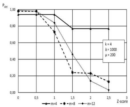
Fig.16. Impact of z-score on the probability of correct diagnosis.