Method of medical images similarity estimation based on feature analysis

Published Online May 2018 in MECS

Medical images similarity estimation is an essential part of modern software tools used in numerous medical investigations including brain researches [1-3]. To develop software tools based on automated processing of images new effective approaches to feature extraction procedure are necessary. It can help to visualize and understand the complex structural and functional organization of tissues. Feature extraction is a complicate task with no universal solution. The research presented in this paper considers contour analysis as one stage of a wider task related to feature extraction techniques in medical images. The test images used in this research are digital images of rat brain slices coloured with different stains. The practical task to be solved within the wider task is the detection of a continuous line that is a feature edge in a rat brain slice. Since test images have different colour gamut, because of different stains used for their preparation, it is necessary to pre-process images in order to enable their uniform representation and, in this way, simplify further search of image edges.

The objective of the research presented in this paper is to develop an effective method for medical images similarity estimation based on features extraction to be used as a part of an automated system of medical image processing and analysis in a wide domain of medical research including brain investigations.

• II.    Related Work

Since the contour analysis is the essential part of the proposed method, comparison of existing methods for contour search has a special value. We consider several effective methods based on active contours, including the following:

• 1.    Method of Active Contour (Snakes) [4];

• 2.    Method of Active Contours Without Edges [5];

• 3.    Method of Minimization of Region-Scalable Fitting Energy [6].

An active contour is a curve that repeats the shape present in the image in maximally accurate way.

Kass et al. [4] introduced a term “snake” that means an energy-minimizing spline locking onto some edge and in this way localizing it accurately. Contours of the snake are represented parametrically as v(s)=(x(s),y(s)) , where x(s) and y(s) are coordinates along the contour and v(s) is the parameterized curve. The energy function is:

^E = f ^Esna_fce ( v ( s ) ) ^d s =

1 f 0

' ^E int ( v ⁽ s ) ) ⁺                '

' ^Eimage ⁽ v ⁽ s ^{)) + E}con ⁽ v ⁽ s ⁾⁾__/

ds ,

where E_int is the internal energy of contour, E_image is the image energy and E_con is the constraint energy [4].

The main point of this method is to find a contour with the minimized total energy.

The disadvantage of this method is that it demands interaction with a user – snakes need to be placed somewhere near the desired contour [4]. That is why all systems which use this method are semiautomatic.

Chan and Vese [5] proposed improved model of active contours that is a basis for their Active Contours Without Edges (ACWE) method. New model enables detection of objects in a given image, based on techniques of curve evolution, Mumford-Shah functional for segmentation and level sets.

The energy function for ACWE is:

F ( c , c ₂, C ) = ц • Length ( C ) + v • Area ( inside ( C ) ) +

+ a L „    “ о ( x , y ) - c J² dxdy ⁺           ,            ⁽²⁾

inside ( C )                                                               ,

+4[       «0 (x,У )-c2,2 dxdy outside(C)

where u 0 is an image, C is any other variable curve, and the constants c 1 , c 2 (depending on C ) are the averages of u 0 inside C and outside C respectively. µ≥0 , ν≥0 and λ 1 , λ₂>0 are fixed parameters [5].

The result of this method is the curve C such that F ( c₁ , c₂ , C ) is minimal.

The advantage of ACWE method consists in that it can automatically detect interior contours starting with only one initial curve and the position of the initial curve is unimportant.

Li et al. [6] presented Minimization of Region-Scalable Fitting Energy method. This method is based on ACWE method, but the important feature of this method is its region-scalability: the authors propose a regionbased model using intensity information in local regions.

A region-scalable fitting energy is defined as follows:

£ ( C , f! ( x ) , f , ( x ) ) =

• ^{= X}1 S o„,s.de (C) ^{K (} x — У )l I ⁽ У ^{) - f (} x )l ^{2 а} У ⁺ ,      ⁽³⁾

• ^{+ X}2 f inside ( C ) ^{K (} x — У )l I ⁽ У ^{)- f} 2 ⁽ x )l ^{2 Й} У

where I is a given vector valued image, C is a closed contour in the image domain, K is a nonnegative kernel function, f 1 , f 2 are two values that approximate image intensities inside C and outside C respectively, λ 1 and λ 2 are positive constants [6].

The comparison of these methods enables concluding that Minimization of Region-Scalable Fitting Energy method is the most quick and accurate in search for contours of an image.

Active contour models are presented in [7, 8, 9]. In particular, Hui Wang et al. in [7] propose an active contour model and its corresponding algorithms with detailed implementation for image segmentation.

An application of active contour models and segmentation algorithms to images are discussed in [10, 11, 12]. The research presented in [13, 14] is focused on an application of active contour models and segmentation algorithms to medical images processing.

• III.    Method Description

The problem of searching for features on a medical image concerns the fact that they are not clear and have many thin and almost invisible borders. We propose the approach which can help to solve this problem.

The proposed method consists of the next procedures:

• 1.    Colour model conversion;

• 2.    Image normalization;

• 3.    Anti-noise filtering;

• 4.  Contours search, conversion, and analysis;

• 5.  Feature analysis.

In the next sections we explain every procedure.

• A. Colour Model Conversion

Input images are mostly coloured images represented in RGB model [15]. It means that every image is described by 3 matrices of equal size: a matrix of red components, a matrix of green components, and a matrix of blue components. To simplify image processing, we convert the coloured image into a grey-scaled image represented by one matrix which is a matrix luminance. The conversion is fulfilled according to following formula:

S,, = 0.2989 X R_n + 0.5870 x G„ + ij                               ij                              ij

+0.1140 x Btj, where Sij is a grey-scaled value, Rij is a red component value, Gij is a green component value, Bij is a blue of the

component value, i and j are indices, 0, 0, M and N are the image sizes.

The resulted grey-scaled image keeps all the features and contours important for further analysis, however, it enables simplification of the image processing procedure.

• B.    Image Normalization

Input images in general and white areas surrounding the tissue image in particular can differ significantly in their size. This difference complicates comparison of images in some set submitted for analysis. To overcome this difficulty the input images should be normalized in their size.

The normalization procedure includes two steps:

• 1.    The cropping of the input image.

• 2.    The resizing of the cropped image.

The image cropping means the removing of its useless parts outside of the tissue image end points on the left, right, bottom, and top. It can be done by using the following algorithm that finds limits i_min , i_max , j_min , j_max of the meaningful part of the image:

• 1.    The grey-scaled image S is converted to a binary image B according to the given threshold T ( 210for rat brain images, T=220 by default).

• 2.    Starting from the first row ( i=1 ) the sum of elements for every next row ( i=i+1 ) is calculated until the following condition (5) is true. Then i min =i .

• 3.    Starting from the last row ( i=n ) the sum of elements for every next row ( i=i-1 ) is calculated until the condition (5) is true. Then i max =i .

• 4.    Starting from the first column ( j=1 ) the sum of elements for every next column ( j=j+1 ) is calculated until the following condition (6) is true. Then j min =j .

• 5.    Starting from the last column ( j=m ) the sum of elements for every next column ( j=j-1 ) is calculated until the condition (6) is true. Then j max =j .

• 6.    The cropped grey-scaled image S cropped =S(i min :i max , j min :j max ) .

m

E B y >  0.                 (5)

j = 1

n

E B j >  0.                  (6)

i = 1

As a result of the cropping procedure, the meaningful image of a minimal size is obtained.

The resizing procedure means the scaling of the image from its initial size ( n×m ) to the size of a given template ( n template ×m template ). This procedure has practical value only if n template , m template – in general case the input image has high resolution (a typical image size is 37000×27000 ) what leads to sufficient increasing of the processing time. To decrease the necessary time, the size

of image can be decreased. The experiments have shown that the decreasing of the image size in 25-28 times (e.g. to the size 1466×964 ) is sufficient.

The resizing procedure implies elimination of redundant rows and columns in the image matrix according to the coefficients:

k =

n

n template

and k_m

m

m template

where operator [] means rounding of a number.

For example, k_n=25 and k_m=28 mean that we keep every 25^th row and every 28^th column (meaningful values are on the cross of them) and abandon the rest of rows and columns. To avoid loss of the image refinement, the meaningful values can be calculated with consideration of a minimal, a maximal, or an average value among redundant values.

As a result of the resizing procedure, the image of the template size is obtained.

Thus, the image size normalization algorithm is resulted in obtaining the image modified in its size according to some given template.

С. Anti-Noise Filtering

In general case significant contours in the image are surrounded by multiple elements like groups of dots and fragments of lines. These elements are meaningless for further analysis and can be considered as noise that should be removed by anti-noise filtering.

The filtering procedure used in the proposed method is based on two-dimensional median filtering [16]. The main idea of two-dimensional median filtering consists in the following.

Let S be a matrix of the image to be filtered:

	s 11	s 12	s 13	s 14	s 1 m
	s 21	s 22	s 23	s 24	s 2 m
s =	s 31	s 32	s 33	s 34	s 3 m
	$ 41	s 42	s 43	s 44	s 4 m
	v s n 1	sn 2	sn 3	• • •           • s n 4	• •   snm J

At each step of the filtering procedure sub-matrix w of the matrix S by size k×l ( k, l) is processed. For example, if k=l=3, then:

w

^s 11

s 21

v s 31

s12

s22

s32   s33

The matrix w 11 is transformed into the vector:

v    ( s 11 s 12 s 13 s 21 s 22 s 23 s 31 s 32 s 33 ) "

Then the elements of the vector v₁₁ are ordered in ascending order. For example, let it be as follows:

v sorted    ( s 22 s 11 s 12 s 23 s 13 s 31 s 21 s 33 s 32 ^{) .}

The middle element of the ordered vector v¹ sorted in our example is s 13 . This element is the median of the submatrix w 11 . Finally, we replace the central element of the sub-matrix w¹ by the median s 13 :

w ¹

median

s 21

v s 31

s12

s13

s32   s33

These steps should be repeated for every element of the input matrix S (the “window” sub-matrix w is moved by 1 element each time). As a result of median filtering, the image purified from small elements (noise) is obtained.

In the proposed method the median filtering procedure is repeated iteratively. The number of iterations and the “window” size k×l are changeable parameters.

For processing only significant contours, we removed all the small pieces from our list of contours. As a result, we are going to process only large objects on image. The parameter of a piece size is changeable.

As a result of the anti-noise filtering algorithm, the filtered list of contours is obtained.

• D.    Contours Search, Conversion, and Analysis

To extract image feathers, we used the modified method of Minimization of Region-Scalable Fitting Energy for ACWE [5, 6]. The main modification consists in conversion of a found contour in SVG-based vector format.

The initial data for the contours search algorithm are the image and the number of iterations for contours search. The larger the number of iterations is, the more accurately contours can be detected. At the same time, the larger this number is, the more time for data processing is necessary.

At the first step of the algorithm a rectangle is set as an initial contour. The following steps are fulfilled at each next iteration of the algorithm [6]:

When all the iterations are carried out, the curves detected in the image are to be separated and then converted into the vector format. It is necessary for further comparison of contours (features) present in both the template image and the image to be analysed. To make this comparison more effective, the number K of vertices in vectorized contours should be equal. Thus, K is determined as a given parameter. Then the detected curve is divided into K+1 fragments and each fragment is substituted by a line of an appropriate length. This procedure is to be carried out for every detected curve.

As a result of both contour search and conversion, the list of vectorized contours (defined by their vertices and lines between them) is obtained.

Next, the contour analysis is fulfilled. It allows us to consider each contour, depending on its location and shape, and in this way it enables finding the conformity of found contours to the given template of features.

As a result, we got the list of contours of image features with advanced information such as a position and a name.

• E.    Feature Analysis

The feature analysis procedure allows us to compare a ration for the estimation of the conformity of found contours to the given template of features.

Let us consider two vectorized contours – C 1 (the feature template) and C 2 (the found contour). Every contour consists of K vertices and K+1 lines (edges) between them. The contours may differ in both positions of their vertices and length of edges and, in this way, they differ in their shape. To estimate the difference or vice versa the conformity of the feature template and the found contour the ration R is calculated:

n ■ Icos ( a ) - cos ( a )l

R = 1--¹,         (13)

2p where α1 is the angle between two adjacent edges of the contour C1; α2 is the angle between two adjacent edges of the contour C2; φ is a measure of the conformity defined as a maximum allowed angle between corresponding adjacent edges in two given contours (the feature template and the found contour) that enables consideration of these contours as visually similar.

Since the most of contours are closed ones, their analysis along with the calculation of the ration R can be started with K initial points. To find the best case for the comparison of the feature template and the found contour, the ration R_k is calculated for L possible combinations of corresponding adjacent edges in two given contours (the feature template and the found contour). The final value of R res is defined as follows:

R res = max ( R 1 ,R 2 , _ , R l ) ,            (14)

where L=K² is a maximum quantity of possible combinations of the corresponding adjacent edges in two given contours if every of them consists of K vertices.

As a result of the feature analysis, the best ratio is obtained for the analysed image according to the given feature template.

• IV. Expert Evaluation Approach

To assess the proposed method, the expert evaluation was used. The evaluation was blind in terms that an expert did not know the results obtained in the computational way according to the proposed method.

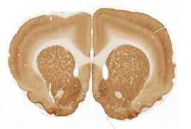
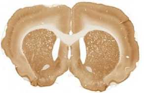
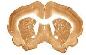
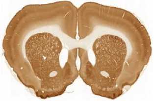
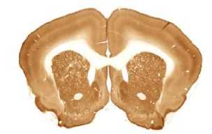
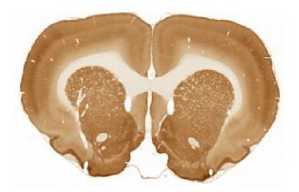
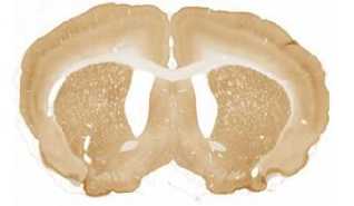
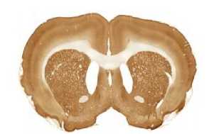
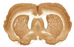
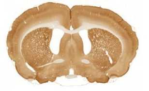
The limited set of 10 images (Fig. 1 and Fig. 2) was used for illustration of the method work in this paper. Since the image presented in Fig. 1 has high quality and the main feature, Corpus Callosum , is clearly presented there, this image was used as the template for feature search. All images in the set were obtained at the same experiment; it means that the same stain was used for brain tissue slices colouring.

A

D

G

B

C

E

F

H

I

The ranking of similarity to template and estimation of degree of similarity was fulfilled in the following way.

The internal structures of images A – I (Fig. 2) were used as a primary criterion for the comparison with the template image. The shape of external boundary is taken into consideration as a secondary criterion. The comparisons were primarily performed side-by-side. Overlay of images was used as a secondary aid.

• A. Ranking

The comparison of the images in first row allows an expert to assert that B more similar (>) to the template than C, which in its turn is more similar to the template than A, giving B > C > A (Fig. 1, Fig. 2). The results for all rows are the following:

• -    First row: B >  C >  A ;

• -    Second row: F >  D >  E ;

• -    Third row: G >  H >  I .

The comparison of the highest ranked in each row, i.e., B , F , and G : F is ranked as the image being most similar to the template.

Excluding F , the comparison of the remaining images of the highest rank in each row, i.e., B , D , and G allows the expert to conclude the following: B is ranked as the image being second most similar to the template.

Excluding F and B , the comparison of the remaining images of the highest rank in each row, i.e., C , D , and G : D is ranked as the image being third most similar to the template. Excluding F , B , and D , the comparison of the remaining images of the highest rank in each row, i.e., C , E and G :

• -    G >  E ;

• -    C >  E .

Deciding between G and C is difficult, since they are quite different in their internal structures. The third ventricle is small in C and large in G . The difference to the ventricle size in the template is about the same for both C and G . Similar considerations apply to other aspects of internal structures. Therefore, G and C are ranked equal as being the fourth most similar to the template. Excluding F , B , D , G , and C , the comparison of the remaining images of the highest rank in each row, i.e., A , E , and H :

• -    E >  H ;

• -    A >  H .

Deciding between E and A is difficult, since they are quite different in their internal structures. The third ventricle is small in A and large in E . The difference to the ventricle size in the template is about the same for both E and A . Similar considerations apply to other aspects of the internal structures. Following overlay of each image to the template, A is ranked before E : A >  E , after G = C .

The ranking between H and I were already decided, thus, H >  I after A >  E .

Therefore, the summary of results of ranking of the images from most similar to less similar to the template, in the side-by-side comparison is the following: F >  B >  D >  G = C >  A >  E >  H >  I .

• B. Degree of Similarity

The estimation of a degree of similarity, from 1 (images are identical) to 0 (images have no similarity), was fulfilled. Overlay of the images was used to estimate the degree of similarity.

In estimating the degree of similarity, the range to be

used would first have to be decided.

Image I (Fig. 2) is the image which is the most different from the template. However, image I is not very different from the template. As an approximation, image I is set to the value 0.75.

Image F (Fig.2) is the image which is most similar to the template. As an approximation, image F is set to the value 0.97.

The summary of estimation of a degree of similarity to the template, based on range 0.75 (least similar) to 0.97 (most similar) overlay of images is given in Table 1.

Table 1. Expert Evaluation

Image Code	Expert Estimation
F	0.97
B	0.92
D	0.88
G = C	0.85
A	0.82
E	0.79
H	0.76
I	0.75

V. Results and Discussion

For validation of the method results the expert evaluation was obtained (Table 2). The results of computed similarity rates and expert's similarity evaluation are slightly different. The main cause of this is that the method does not enable to separate Corpus Callosum from the holes beneath it. During the expert's evaluation, these holes are not considered. At the same time, they are important for the method.

Another issue is that an expert is not so attentive to small but important graphical details (separate dots, combination of colours, slight changes of a colour level, etc.) as the computer program is, but solving this issue is out of the research scope.

For the analysis of the obtained results the coincidence degree C (in %) was calculated for each pair “Computed Rate” - “Expert Evaluation” (Table 2) according to (15).

C = ^

R

comp

R

eval

R

eval

R

comp

■ 100%,

■ 100%,

Rcomp   Reval

R^ ^ R comp

where R_comp is a computed rate for a given image, R_eval is an expert evaluation for the same given image.

The coincidence degree for the template image

The average coincidence degree for the rest of images is 87%. Therefore, the results obtained from the proposed method can be considered as good.

b

a

d

f

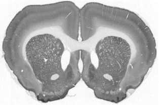
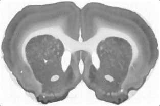
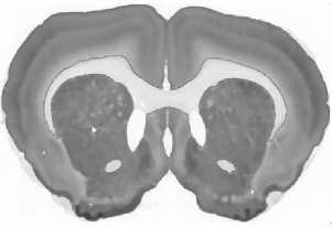
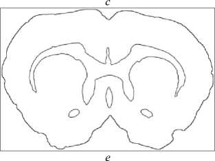
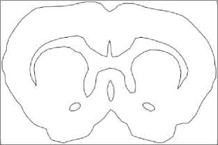
Fig.3. Stages of an image processing: a – original image, b – gray-scaled image, c – image after anti-noise filtering, d – contours search result (red lines), e – vectorized image, f – smoothed vectorized image.

Table 2. Evaluation of the method results

File Name	Image Code	Computed Rate	Expert Evaluation	Coincidence Degree, %
img_01_01.png	template	1.00	n/a	n/a
img_01_02.png	A	0.79	0.82	96
img_01_03.png	B	0.77	0.92	84
img_01_04.png	C	0.78	0.85	92
img_01_05.png	D	0.88	0.88	100
img_01_06.png	E	0.78	0.79	99
img_01_07.png	F	0.78	0.97	81
img_01_08.png	G	0.65	0.85	77
img_01_09.png	H	0.59	0.76	78
img_01_10.png	I	0.56	0.75	75

• VI.    Further Work

The proposed method includes the procedure of conversion from a RGB model image to a grey-scaled image in order to simplify further processing. However, better results could be obtained if analyse every colour matrix (red, green, and blue) separately and then choose the best case from three options.

Depending on the stain type images in an experimental set differ not only in size and position, but also in their brightness and colour hue. Thus, better results can be achieved if we normalize not only geometrical characteristics such as size and position, but also consider visual characteristics of the image, namely its brightness and colour hue, in the image normalization procedure. The brain tissue image adjustment method [20] can be used for this purpose.

A smarter algorithm – seam carving algorithm [21] – that supports content-aware image resizing can be employed for the image cropping in image size normalization procedure.

The processing of images in high resolution can lead to better results. The increasing of processing time can be overcome by parallel programming.

• VII.    Conclusion

The proposed method of medical images similarity estimation allows us to assess similarity of a given image and a given template taking into consideration the core elements of the medical image. The method can be used for automated medical images pre-processing in a wide range of medical researches. The analysis of the proposed method allows us to conclude that the accuracy of the assessment varies from 75% to 100% comparatively to a human expert estimation.

• VIII.    Acknowledgements

The authors acknowledge Professor Jan G. Bjaalie, Head of the Institute of Basic Medical Sciences at the University of Oslo, Norway, for the expert evaluation of the proposed method.

The essential part of the research has been carried out within the EUMLS project funded by Marie Curie Actions – International Research Staff Exchange Scheme FP7-People-2011-IRSES (project number is 295164) for giving the opportunity to fulfil this research.