Mimicking Nature: Analysis of Dragonfly Pursuit Strategies Using LSTM and Kalman Filter

Predator and Prey pursuit is a natural phenomenon that is very common in animals. A predator is a living body or animal that hunts and consumes something to feed itself. On the other hand, Prey is that target which is hunted by Predator as it’s food. The event when a Predator chases its Prey to catch the target is known as pursuit. The chase starts either with prey or from predator and ends after either capturing the prey or escaping prey away. In the earth, there are lots of Predators who chases and kills their Preys to feed themselves and their children. It is a natural principle that a Predator will try to pursuit a Prey as soon as the Predator notices a target and gets a chance for a successful hunt. Whereas a Prey will try to escape from the Predator as soon as it learns something is behind the Prey to hunt it. So, basically, Predator motive is capturing the prey running away and not being captured by predator is motive of prey. Pursuer and evader in existence usually equate to attacker and victim, respectively; they may be autonomous machines in an artificial environment. Evaders succeed in many forms, e.g. the survival of a specific evader is vitally necessary in combination to combat a single pursuer or group of pursuers most frequently. A pursuer typically moves quicker than the intended evader, for example the cheetah is the supreme cursorial pursuer[1]. Each predator has a particular objective of catching prey. Each method of predator movement varies by the type of predator. Every predator has their own way of hunting prey.

A predators’ efficiency enhances when it chases different types of preys[2]. A predator learns the movements of different types of prey while chasing them. Study has shown that the predators who communicate with genetic algorithms have evolved considerably more effectively. The development of both prey and predator is driven by predation failure[2]. Both adjust their movements for the next time to fix their faults for being successful. Typically speaking, predators would prefer resource rich areas and avoid places with high chance of predation. A hunter will also aim to balance the period the prey spends in resource-rich areas to increase the likelihood of catching prey. This study assesses artificial actions of predators and prey and compares them to actions generated from biological theoretical models[3]. Specifically, the amount of time expended on food patches by predators and prey agents is calculated. To contend with each other for the purpose of predator-prey behavior, where each species strives to learn the most acceptable behavior. For intruder members, one group adapts habits, while the other adapts habits for predators. The role of pursuit-evasion includes the apprehension of one predator-agent [3]. Capture of Prey takes place while a Predator enters the same grid cell as the Prey. The hunter pursues the Prey, and the Prey evades the trap, foraging wealth areas to obtain food. Pursuit predation centers around a distinct pattern of activity between predator and prey; predators will travel along with them while prey migrate to locate new foraging areas. Predators concentrate in places with large prey abundance, and so prey will avoid such regions. Pursuit-evasion of both the human and the technological universe is interesting. Usually, though possessing less flexible maneuverability, a pursuer moves quicker than the intended evader. A quicker pursuer normally has fewer agile tactics, i.e., as it moves at a greater pace, it has a wider turning range, whereas an evader may have more flexible (rapid turning) tactics to prevent detection. An evader’s escape strategy which takes advantage of this is essentially necessary for survival[1]. In the actual world approach the Predator activity becomes more accurate. The risk activity is similar to the attacker and less nuanced in good real life[4].

The main objective of this research is to find out the strategy and all the dependencies of the pursuit strategy of a certain Predator of catching its prey along with the strategy of how the Prey tries to evade from being hunted. The Dragonfly also known as the natural drone had been considered as the Predator in this research because the success rate of a Dragonfly catching its prey is around 95% [5] .Flies had been considered as Prey because most often dragonflies prefer flies to pursue, and flies are easily available to find. The motivation of this research is to extract the strategy of dragonfly’s’ chasing after a fly, analyze the tactics, understand the strategy, and build up an algorithm based on that strategy. If that algorithm is applied to any programmable UAV for example Drones, Missiles, Torpedoes, etc., their chance of hitting the target will be as same as that of a Dragonfly. So, the pursuit will be more reliable, efficient, and accurate.

In this section, some research questions have been listed with respective objectives. These questions led the research to reach the main objective. They helped the researchers to find and select necessary articles related to this research to review. Besides, they guided effectively to find the appropriate research method to follow. The questions have been listed below:

• •    What Strategy(s) does a predator follow to go after its prey?

• •   In which period does a predator try to pursue the prey?

• •   Does the initiation point depend on Time or Distance or Both?

2.    Literature Review

The objective of the first question is to find out the strategy of a predator’s attack. The objective for the second question is to find out the attacking initiation point. The objective for the third question is to find out the dependencies of attacking strategy.

Unmanned aerial vehicles (UAVs) are becoming more and more prevalent because of technological advancements. Due to its wide range of adaptability, simple installation, and very low operating costs. UAVs have been using in numerous sectors of advancement such as rescues [6] and surveillance [7], monitoring [8], emergency document delivery [9] and tracking [10]. Researchers have been investigating and developing evolutionary bio-inspired algorithms to optimize UAV’s performance. Swarm Intelligence based UAV path planning algorithms such as NPSO, IPSO, DPSO, MOPSO are Particle swarm optimization (PSO) based algorithm and GM-ACO, ACO, MMAC are Ant Colony Optimization (ASO) based algorithm. There are also hybrid algorithms, behavior-based algorithms, and Bio-Inspired Neural Network (BINN) based algorithms making potential contributions to solve the optimization problems[11]. The Flying Ad hoc Network (FANET) [12] is a wireless network that operates autonomously and consists of clusters of unmanned aerial vehicles (UAVs) that interact with one another. Motion planning algorithms [13] are being applied to UAV to minimize the costs and increase efficiency.

The majority of conventional UAV navigation algorithms are unable to converge because of the large volumes of interactive data in extremely dynamic situations with plenty of moving objects [14] also performance is hampered by the inability of current UAV navigation algorithms to detect motion and choose the optimal UAV-ground linkages in realtime [15]. Size, weight, and power limitations are other challenges for real-time obstacle identification for UAV navigation[16]. Now days researchers are in search of optimal solution flowing hybrid approaches like combining motion planner and Deep learning approaches[17] , PPO-based Reinforcement Learning for UAV Navigation[18]. The analysis of our study could lead researchers to increase the optimization accuracy.

The kinematics of predator–prey relationship varies hugely. It depends on the medium in which they take place and on the motor and sensory systems of predator and prey. Generally, predators hunt different types of prey. Predators apply one of its behavioral strategies with speedy movement or they create their own hunting method for each type of prey. Prey vary survival tricks and its sensor’s motor abilities [19].

In addition to the descriptive mechanisms of natural interaction of predator – prey, very few papers have likened the working power of predators to ensuing different kinds of prey. Also, prey is being followed by a variety of types of predators. To ordain how the combination of predator – prey vary from one another will help to express how general predator – prey inter-linkage is and how much the mechanism studies of a single predator–prey pair can be anticipated [20].Generally, if the density of prey is increased, predator hunts and eats more unit number of prey until some satiation point is reached. After that the rate of eating is constant when the number of eating prey is above the satiation point. It is possibly due to the time dependent physical limitations of prey hunting and eating. It is called functional response. Then if a good number of preys is accessible for an adequate time, the total number of presence predators rises. It is called numerical response. These two kinds of response can happen differently or together [21].

Dragonflies are renowned for their predatory abilities and for their realization of comprehensive diversity of flying prey. Working power at predating is troublesome for dragonflies. The capability power of predating of both male and female dragonflies are directly affected by the gain in mass. If any means male or female dragonfly spend more time for searching, it can sustain for grown mortality due to the risk of being attacked while hunting and territorial species risk while dragonflies are seized with the hunt and stirring of prey [20].

In an experiment the result shows that prey catching success and efficiency both decrease with increasing size of prey. Average prey speed rises with size. Dragonflies get going on hunting large size prey when they are located far from the prey. The total distance of the dragonflies is correlated with the distance of the prey. If the larger prey distance is too more, it may be a limitation for dragonflies’ visual perception. Dragonflies may be incapable of catching larger prey flying very close to their perch. Predator-prey interaction is a natural behavior. To know all about predator-prey interaction requires elaborate knowledge not only of locomotory mechanics but also sensory abilities and limitations of both predator and prey[20].

After data analysis it is realized that the length of time of predator’s pursuing is both variable and adjustable. An extent of the optimal diet model which includes adjustable pursuit times to forecast the length of time that a predator should pursue their prey. The model has three important factors, and these are if the number of strong preys is increased, the defective prey should serially depart from the diet. Then the second factor is the model creates patterns of frequency dependent and inverse frequency dependent preying depending on the how the encounter rates of prey varied. The last factor is the consistence of defective prey can impact the proportion seized of more strong prey [22].

• [23]    investigates sensorimotor control in dragonflies during prey interception, akin to vertebrate reaching behavior. Tracking the dragonfly's head and body movements reveals the use of predictive models for both the insect's body dynamics and prey motion. Evidence suggests that forward and inverse models guide interception steering, with continuous predictive rotations of the dragonfly's head tracking the prey's angular position. The head-body angles, established through prey tracking, contribute to systematic rotations aligning the dragonfly's body with the prey's flight path. The study highlights the computational sophistication of insect behavior, showcasing the integration of internal models in guiding interception maneuvers while relying on vision for responses to unexpected prey movements.

3.    Research Method

Some rules are used by animals to establish behaviors. Those rules are named as triggers which ordains when the behavior starts. These selected rules are also a scope to initiate sensorimotor constraints that impact how to end the behavior. These constraints are especially important in impacting success in prey capture. When dragonflies lead up to take off and land, they use a order of sensorimotor rules that ordain the time of takeoff and increment the probability of successful capture. At first a head saccade is made by dragonflies following soft pursuit movements to position the direction of its eye at the targeted prey. Then the dragonflies evaluate the angular size of prey and the speed of prey within a range of favored area. Finally, the time is reached when dragonflies take off and just then the prey will cross the zenith. The all actions which have been described assist a goal. The angular size speed influences the dragonfly’s flight to the targeted prey. In this time the dragonfly’s head movements and the forecasting takeoff assures flights starting with the prey which is visually in still and directly above the level of head. Generally, prey does not invoke any takeoff. Commonly at least one of the criterions is failed by it and the overhead positioning or the loss of prey’s stabilization which are sharply correlated with the terminated flight. So, from plenty of strong target, a set of takeoff which is conditionally based on the prey and body states are chosen by dragonflies and it is continued most likely to the end to ensure a successful attack to capture [24].

Study of [25] delves into the sophisticated reflexes of dragonflies, unraveling the intricate mechanisms involved in their mid-air righting abilities. Through kinematic analyses, physical modeling, and 3D flight simulations, the research uncovers that dragonflies utilize left-right wing pitch asymmetry to execute a rapid 180-degree roll, recovering from an upside-down position in approximately 200 milliseconds. Experiments with blocked vision indicate that this maneuver is initiated by the dragonfly's ocelli and compound eyes, revealing a direct pathway from the visual system to the wing-pitch regulating muscles. The developed methods provide quantitative tools for deciphering internal actions in insects' acrobatics, with broad applicability to understanding natural and robotic flying systems.

An investigates of pursuit behavior [26] in the context of predator–prey interactions, focusing on the unique foraging strategy of Corynorhinus townsendii , Townsend's big-eared bat. Unlike high-speed, open-area foragers, this species employs slow and highly maneuverable flight near vegetation. The analysis of 44 successful captures reveals that C. townsendii relies primarily on a stealthy approach, successfully capturing prey in 32 out of 44 trials. When the initial approach falls short, the bat adapts its pursuit strategy by combining pure pursuit and proportional navigation, demonstrating a flexible and adaptive approach to capturing prey in its distinctive ecological niche.

An innovative method [27] of optimization that takes cues from the biological sight system—specifically, the mechanics of the dragonfly. It creates a neural network model by combining these revelations with the ideas of swarm evolution. When given grayscale photos as input, this model produces a variety of global learning rates that provide a population evolution-style approach to finding global optima in complex optimization problems. The competitiveness of this method is demonstrated by comparative tests, which also indicate that it is useful in building an operational amplifier and solving high-dimensional benchmark suites. Considering all the things, it is a promising combination of computational concepts with biological inspiration to address challenging optimization problems.

In conclusion, this thorough study delves into the complex dynamics of predator-prey interactions, specifically highlighting the methods and techniques used by different species, such as dragonflies, to become predators. The research mentioned provides insight on the complex nature of these interactions by examining the kinematics, sensorimotor control, and pursuit behaviors of predators such as dragonflies, along with the reactions and adaptations of their prey. Furthermore, the investigation encompasses novel techniques for optimization motivated by biological visual systems, demonstrating the possibility of incorporating biological knowledge into computational methodologies. This thorough analysis offers insightful information and opportunities for more investigation into the dynamics of predator-prey relationships, particularly considering the research goals focused on comprehending predator attack techniques, initiation points, and dependencies.

Predator Prey Pursuit system concept has been previously used in a plethora of ways. This model has been also used in neural networks and different types of algorithms. Meta-heuristic algorithms are inspired by distinctive common perspectives. Learning from nature to fathom issues got to be valuable as nature finds solution for issues without being told. Both predators and preys are interaction has advanced for long. It implies that the predators have overseen to capture the frail or unfortunate prey to outlive additionally the preys have overseen to outlive. There are diverse sorts of predators and prey interactions. Among those intuitive, the interaction in which the predators run for pursuit their prey motivates the prey-predator algorithm. These intelligent have persuaded distinctive calculations. For case, spurred by the interaction between a predator and its prey.

In this section, the methodology of the research starting from Data collection to the end has been described. The research had been performed using 2-dimensional (2D) data. For research purposes an image annotation tool Labelme, python 3 with lots of libraries and jupyter notebook has been used.

• 3.1.    Data Collection and Formation

• 3.2.    Data Preprocessing

• 3.3.    Finding Velocity and Distance over Time

For data, some video clips had been used where the event of Predator chasing a Prey had been recorded. There were 5 sample videos. The videos had been collected from [23] 4 samples and another 1 from online source[28]. Several frames had been extracted from those videos. From each sample we had split video frames for the analysis. Using an image annotation tool Labelme, the predator and prey had been annotated from each of those frames as two different objects. After that, Labelme provided one JSON file for each frame. Those JSON files contain the information of each respective image frame. The JSON files also contained the coordination of both Predator and Prey in distinct timespan. These JSON files had been used for the next steps of research method. For demonstration purposes figure 1 shows the raw clips and annotation formulation from sample 1 video.

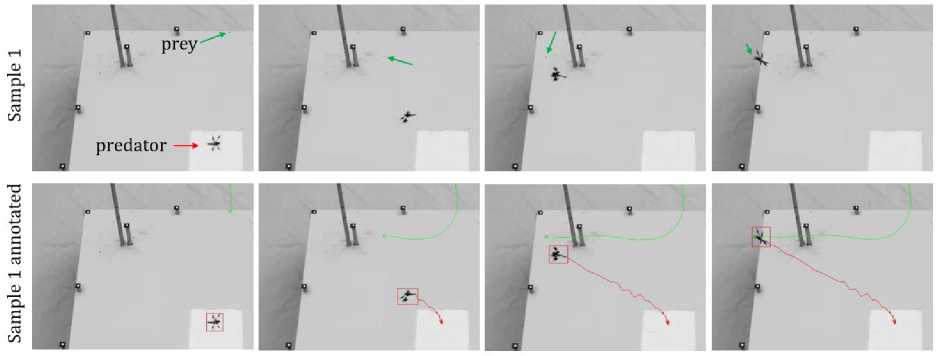
Fig.1. Four extracted frames from raw video sample 1 (top) and corresponding annotated bounding box and tracking path (bottom) of both Predator (red) and Prey (green)

There were not equal number of JSON files in sample. They vary because every video clip was not equal in time length. This inequality could cause trouble while analyzing data. To prevent this problem, interpolation techniques had been used to generate more data using existing data and created 109 data for each sample to bring them up in the same scale of data points. For interpolation, the linear spline method had been used. For further data processing, the Moving Average Filter algorithm had been used to reshape those data so that the curve gets smoothen enough for easy analysis.

For strategy analysis, both Predators and Preys velocity and their internal distance over hunting timespan is crucial. So, find out the velocity over time the JSON files have been used. The different co-ordinates of both Predator and Prey had been fetched imported. This task had been done using python script. From those co-ordinates, the distance between each co-ordination had been extracted using Euclidean distance formula to find out the trajectory.

distance = 7(^ 1 -^2) 2' +(^ 1 —4) 2 (1)

After getting the list of distances, the velocity had been extracted. In this case, the acceleration was unknown, and it might also be dynamic. So, velocity had been fetched using distance and time. The distances were fetched earlier but for the time, the time length of a video had been taken and divided by the total number of JSON files for each sample. Thus, the constant travelling time from one co-ordination to another co-ordination had been found out. By the set of distances and the time, the set of velocities of both Predator and Prey had been extracted from the whole hunting and evading journey.

^ = f (2)

For each distance travel, the velocity of both Predator and Prey had been extracted and listed in two separate lists. The problem was their unit was not standard. It was in pixel measurement. To get the standard unit, the pixel unit had been converted into centimeters using the formula given below.

centimeter = ^^ * 2.54 (3) dpi

Here, dpi means pixel density or more specifically dots per inch. Most of the cases, the dpi is 96. So, 96 dpi means 96 dots or 96 pixels per inch. On the other hand, 1 inch = 2.54 centimeter. So, the formula stands as equation 3 mentioned above. After that, the distances over time between both Predator and Prey had been extracted also using equation 1, the euclidean distance formula.

Next the preprocessing part had been performed described in 3.2 for good and easy analysis. Using all the data, two separate garphs had been plotted using pyplot from matplotlib library for Velocity-Time analysis and Distance-Time analysis.

• 3.4.    Application of LSTM Algorithm

• 3.5.    Application of Kalman Filter Algorithm

4.    Results

• 4.1.    Speed and Distance Analysis over Time

Recurrent neural networks are a strong form of neural network intended to deal with pattern dependency. Here the recurrent neural network used in deep learning is the Long Short-Term Memory Network or LSTM Network [29], as it is possible to accurately train very large frameworks.

In this research, the LSTM algorithm had been applied to get the strategy model using the deep learning library of Tensorflow and Keras in python. Among all the data, 70% of data had been trained to get the model and the rest 30% data had been used for testing the model. Tensorflow and Keras were utilized to apply the LSTM calculation. The mean square error between the actual data and the LSTM model observed had been discovered for the analysis purpose. All the data were plotted separately in separate graphs.

The Kalman filtering algorithm [30] helps us to predict the position of an object based on observations or measurements. For object tracking, intelligent navigation systems, economic prediction, and different types of applications the Kalman filter algorithm plays a vital role. Using the previous information of the state it produces a forward projection state or predicts the next phase which is the fundamental assumption of the Kalman Filter.

In this research, the Kalman filter formula had been applied to track the direction of both Predator and Prey to discover whether the Kalman fliter could trace the trajectory of both Predator and Prey. To do this, the pykalman library had been used. After that the actual trajectory and the Kalman out had been plotted for further analysis.

In this section, the results of experiments discussed in section 3 have been shown and demonstrated. For simplicity reason, the results have been explained in 3 subsections for each approach.

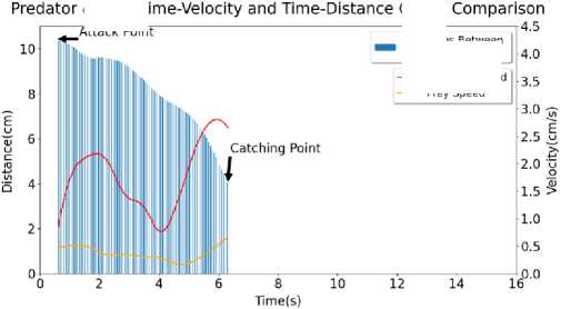
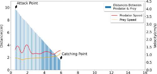
In this section, the results of Velocity, Distance over Time graphs have been disclosed. Each graph consists of two parts. One is for Distance-Time graph annotated by bar chart and another one is Velocity-Time annotated by curves. The bar chart represents the distance between Predator and Prey over Times whereas curve chart represents velocity of Predator and Prey over Times. The attacking point and catching point has been annotated by black arrows.

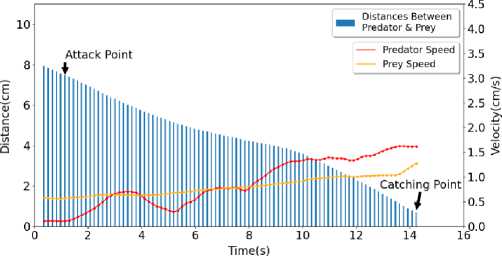
In Figure 2, the graph of Sample 1 has been shown. Here, initial Predator speed is around 0.1067 cm/s, average Predator speed is around 0.8727 cm/s, maximum Predator speed is around 1.6224 cm/s, final Predator speed is 1.6206 cm/s. Standard deviation for Predator speed is around 0.4843 cm/s. Initial Prey speed is around 0.5792 cm/s, average Prey speed is around 0.8034 cm/s, maximum Prey speed is around 1.2748 cm/s, final Prey speed is around 1.2748 cm/s. Standard deviation for Prey speed is around 0.1787 cm/s. Initial Distance is around 7.9231 cm, average Distance is around 4.4387 cm, maximum Distance is around 7.9231 cm, final Distance is around 0.6894 cm. Standard deviation for Distance is around 1.9075 cm.

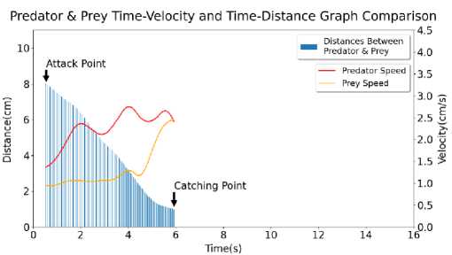
In Figure 3, the graph of Sample 2 has been shown. Here, initial Predator speed is around 1.3702 cm/s, average Predator speed is around 2.2768 cm/s, maximum Predator speed is around 2.7501 cm/s, final Predator speed is 2.4131 cm/s. Standard deviation for Predator speed is around 0.3590 cm/s. Initial Prey speed is around 0.9554 cm/s, average Prey speed is around 1.3109 cm/s, maximum Prey speed is around 2.4395 cm/s, final Prey speed is around 2.4357 cm/s. Standard deviation for Prey speed is around 0.4496 cm/s. Initial Distance is around 8.0252 cm, average Distance is around 4.3680 cm, maximum Distance is around 8.0252 cm, final Distance is around 1.0056 cm. Standard deviation for Distance is around 2.2927 cm.

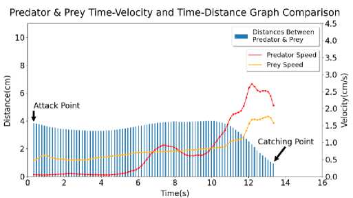
In Figure 4, the graph of Sample 3 has been shown. Here, initial Predator speed is around 0.0624 cm/s, average Predator speed is around 0.7584 cm/s, maximum Predator speed is around 2.7284 cm/s, final Predator speed is 2.0918 cm/s. Standard deviation for Predator speed is around 0.8268 cm/s. Initial Prey speed is around 0.4726 cm/s, average Prey speed is around 0.8129 cm/s, maximum Prey speed is around 1.7691 cm/s, final Prey speed is around 1.5764 cm/s. Standard deviation for Prey speed is around 0.3505 cm/s. Initial Distance is around 3.8333 cm, average Distance is around 3.3922 cm, maximum Distance is around 3.9955 cm, final Distance is around 0.9369 cm. Standard deviation for Distance is around 0.6924 cm.

Graph

Attack Point

--- Predator Speed

— Prey Speed

In Figure 5, the graph of Sample 4 has been shown. Here, initial Predator speed is around 0.8687 cm/s, average Predator speed is around 1.7692 cm/s, maximum Predator speed is around 2.8082 cm/s, final Predator speed is 2.6711 cm/s. Standard deviation for Predator speed is around 0.6125 cm/s. Initial Prey speed is around 0.4792 cm/s, average Prey speed is around 0.3673 cm/s, maximum Prey speed is around 0.6533 cm/s, final Prey speed is around 0.6533 cm/s. Standard deviation for Prey speed is around 0.1167 cm/s. Initial Distance is around 10.3467 cm, average Distance is around 8.2265 cm, maximum Distance is around 10.3467 cm, final Distance is around 4.0501 cm. Standard deviation for Distance is around 1.6666 cm.

In Figure 6, the graph of Sample 4 has been shown. Here, initial Predator speed is around 1.3301 cm/s, average Predator speed is around 1.2200 cm/s, maximum Predator speed is around 1.6431 cm/s, final Predator speed is 1.2687 cm/s. Standard deviation for Predator speed is around 0.1753 cm/s. Initial Prey speed is around 0.7749 cm/s, average Prey speed is around 0.8037 cm/s, maximum Prey speed is around 1.1007 cm/s, final Prey speed is around 1.1007 cm/s. Standard deviation for Prey speed is around 0.0821 cm/s. Initial Distance is around 9.7596 cm, average Distance is around 5.6178 cm, maximum Distance is around 9.7596 cm, final Distance is around 1.5337 cm. Standard deviation for Distance is around 2.3743 cm

• 4.2.    Speed and Distance Prediction Analysis by LSTM

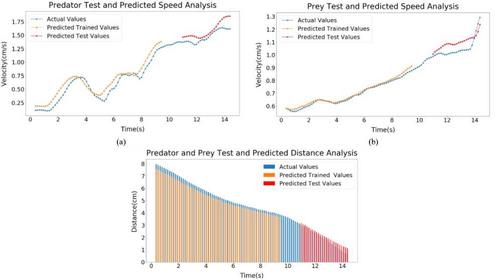
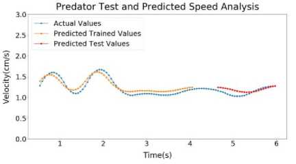
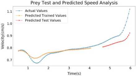
In this section, the output of LSTM model has been disclosed. Each sample has 3 outputs. One for Predator, one for Prey and the last one for Distance prediction. The Predator and Prey graph both are Velocity-Time graph and Distance graph is a Distance-Time graph. After feeding the trained data into LSTM algorithm, an LSTM model was generated. Though the model predicted all the parameters almost correctly, it has some small fraction of errors. The output has been shown by Graphs and all the output plots have their distinguished color annotated inside graph legions.

(c)

Fig.7. Sample 1 test and predicted speed profile (a) Predator (b) Prey (c) Predator and prey distance graph

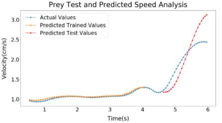
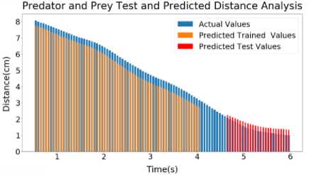
Inside Figure 7(a), LSTM output of Predator of Sample 1 has been shown. Here, the error for Predator Predicted Trained values of speed is around 1.24%. The error for Predator Predicted Test values of speed is around 1.57%. Figure 7(b), LSTM output of Prey of Sample 1 has been shown. Here, the error for Prey Predicted Trained values of speed is around 0.19%. The error for Prey Predicted Test values of speed is around 1.10%. on figure 7(c), LSTM output of Distance of Sample 1 has been shown. Here, the error for Predicted Trained values of Distance is around 0.22%. The error for Predicted Test values of Distance is around 0.79%.

(a)

(b)

(c)

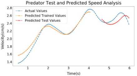
Fig.8. Sample 2 Test and predicted speed profile (a) Predator (b) Prey (c) Predator and prey distance graph

(c)

Fig.9. Sample 3 test and predicted speed profile (a) Predator (b) Prey (c) Predator and prey distance graph

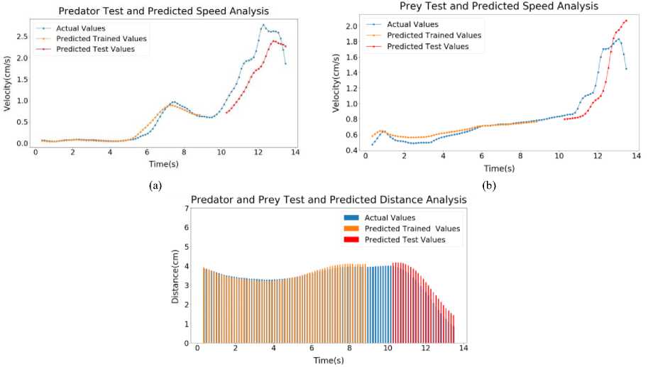
Inside Figure 8(a), LSTM output of Predator of Sample 2 has been shown. Here, the error for Predator Predicted Trained values of speed is around 1.01%. The error for Predator Predicted Test values of speed is around 1.27%. on figure 8(b), LSTM output of Prey of Sample 2 has been shown. Here, the error for Prey Predicted Trained values of speed is around 0.57%. The error for Prey Predicted Test values of speed is around 2.8%. Inside figure 8(c), LSTM output of Distance of Sample 2 has been shown. Here, the error for Predicted Trained values of Distance is around 0.65%. The error for Predicted Test values of Distance is around 1.86%.

Inside Figure 9(a), LSTM output of Predator of Sample 3 has been shown. Here, the error for Predator Predicted Trained values of speed is around 0.93%. The error for Predator Predicted Test values of speed is around 4.88%. On figure 9(b), LSTM output of Prey of Sample 3 has been shown. Here, the error for Prey Predicted Trained values of speed is around 0.28%. The error for Prey Predicted Test values of speed is around 2.69% and figure 9(c), LSTM output of Distance of Sample 3 has been shown. Here, the error for Predicted Trained values of Distance is around 1.15%. The error for Predicted Test values of Distance is around 4.83%.

(a)

(b)

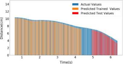
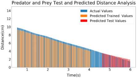
Predator and Prey Test and Predicted Distance Analysis

(c)

Fig.10. Sample 4 test and predicted speed profile (a) Predator (b) Prey (c) Predator and prey distance graph

(a)

(b)

(c)

Fig.11. Sample 5 test and predicted speed profile (a) Predator (b) Prey (c) Predator and prey distance graph

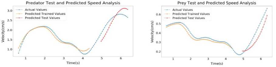
Inside Figure 10 (a), LSTM output of Predator of Sample 4 has been shown. Here, the error for Predator Predicted Trained values of speed is around 2.03%. The error for Predator Predicted Test values of speed is around 3.29%. Inside Figure 10(b), LSTM output of Prey of Sample 4 has been shown. Here, the error for Prey Predicted Trained values of speed is around 0.24%. The error for Prey Predicted Test values of speed is around 0.85%. Inside Figure 10(c), LSTM output of Distance of Sample 4 has been shown. Here, the error for Predicted Trained values of Distance is around 1.4%. The error for Predicted Test values of Distance is around 4.24%.

Inside Figure 11(a), LSTM output of Predator of Sample 5 has been shown. Here, the error for Predator Predicted Trained values of speed is around 1.46%. The error for Predator Predicted Test values of speed is around 0.82%. Inside Figure 11(b), LSTM output of Prey of Sample 5 has been shown. Here, the error for Prey Predicted Trained values of speed is around 0.23%. The error for Prey Predicted Test values of speed is around 0.87%. On Figure 11(c), LSTM output of Distance of Sample 5 has been shown. Here, the error for Predicted Trained values of Distance is around 0.47%. The error for Predicted Test values of Distance is around 2.14%.

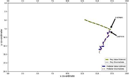
• 4.3.    Kalman Filter Output Analysis

In this section, the outputs of Kalman Filter algorithm have been disclosed. As mentioned earlier, the Kalman Filter had been applied here because of checking that if the algorithm can trace the trajectory of both Predator and Prey.

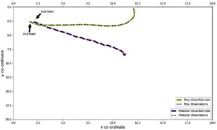
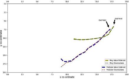
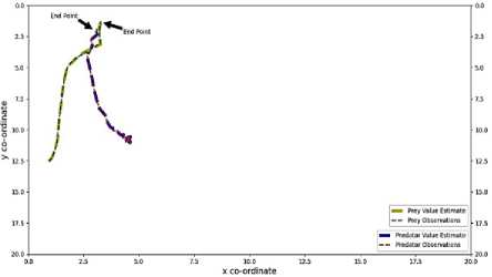
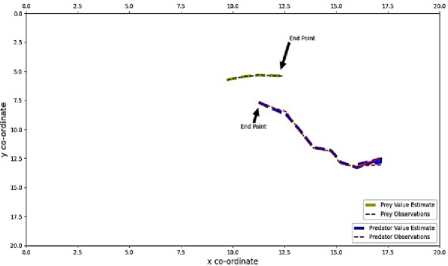
The actual value curve of Predator has been plotted and indicated by red colored dashed line. The estimated value curve of Predator generated by Kalman Filter has been plotted and indicated by blue colored wider dashed line. The actual value curve of Prey has been plotted and indicated by green colored dashed line. The estimated value curve of Prey generated by Kalman Filter has been plotted and indicated by yellow colored wider dashed line. The end points of both Predator and Prey have been indicated by black arrows for better understanding. All the outputs and graphs indicate that the Kalman Filter algorithm successfully estimated the trajectories of both Predator and Prey. Every chase was successful, the trajectories are accurate. A little bit of errors has been disclosed on estimated trajectories which can be negotiable. In this research, for applying Kalman Filter algorithm, pykalman library was used. This algorithm had been designed for constant velocity trajectory tracing. For this this reason when the acceleration had been tuned and made to 0 cm/s, the Kalman Filter algorithm successfully traced the trajectory of both Predator and Prey. Although there were some errors, it was under satisfactory range.

In figure 12 for sample 1, the error for the Predator was around 0.49%, the error for the Predator around was 0.11% For sample 2, the error for the Predator was around 7.43%, the error for the Prey around 0.74%. For sample 3, the error for the Predator was around 0.51%, the error for the Prey around was 0.4%. For sample 4, the error for the Predator was around 1.99%, the error for the Prey around was 0.10%. For sample 5, the error for the Predator was around 4.55%, the error for the Prey around was 0.15%.

(a)

(b)

(c)

(d)

(e)

Fig.12. Kalman filter output of sample 1(a), Sample 2(b), Sample 3 (c), Sample 4(d), Sample 5(e)

5.    Discussion

From the result section, very major clues and information had been gathered that led the researchers to find out the strategy of hunting procedure of a dragonfly and the evading procedure of a fly. The 5 samples were captured from 5 situations. So based on the situation, the attacking time, catching time, environment, speed, distance may vary but there must be at least a single match or at least a single parameter which matches every situation and based on which the dragonfly hunts its Prey.

After analyzing the data, it is found that a dragonfly maintains a certain distance while catching its Prey. When a dragonfly detects a Prey, it first observes the movements of the Prey, then follows the Prey for a certain time. A certain time depends on the distance. Based on the distance the dragonfly modulates its speed accordingly. If the dragonfly crosses the mean distance, it slows down itself and when it lags too far from the mean distance it increases its speed again. It continuously modulates its speed. While balancing the speed, a dragonfly also calculates the movement speed, acceleration possibilities, movement direction of its prey. When the dragonfly completely reads the movements of its Prey while balancing the distance, it rapidly increases enough speed to catch and consume the Prey. From that specific distance, the dragonfly assures itself that it will catch the Prey successfully even if the Prey increases its speed or changes direction. Because the dragon already has drawn the movement pattern of its Prey in the brain. On the other hand, Prey increases its speed when it senses something is trying to hunt it to tries to flee away from the Predator. But the Prey most of the time fails to escape because it can’t detect the predator from the long distance. And the Predator takes this advantage and maintains the safe distance to get the best chance. The time when the Prey senses the Predator, it becomes too late for the Prey to escape. Predators last moment acceleration is always greater than the Prey. Most of the time Prey does not get enough time to accelerate enough to escape from the dragonfly. And this secret strategy leads a dragonfly to the victory of hunting a Prey successfully.

So, the answer to the first question is a dragonfly follows distance maintenance strategy to pursue a Prey. The time when dragonfly reaches to the best distance that will surely lead the dragon to catch the Prey, it increases speed to catch the Prey. The Predator may keep balancing the distance even after getting the best chance to hunt the Prey. And this behavior of dragonfly increases the hunting chance even more. One most important thing to discuss is, here time and distance are not the same thing. So, there is no chance to get confused between time and distance. Predator attacks based on the best distance not the best time. The initiation point is distance in this case and thus it can be said the initiation point depends on the distance. In the case of Kalman Filter, it is already mentioned that the Kalman Filter has been designed for tracing objects having constant velocity. And in the hypothesis, it was analyzed that a Dragonfly tries to keep its velocity constant to maintain the safe (mean) distance. It uses instant acceleration or deceleration to modulate its speed when it goes too close to the Prey or too far from the Prey before the best chance comes. If the errors are checked and analyzed, it can be observed that the error for tracing the Prey is very few in compared to the Predator. This happens because the Prey, before sensing the Predator, moves in a constant velocity and very little acceleration whereas the dragonfly has little bit higher error because of their frequent acceleration and deceleration. So, this output of Kalman filter confirms the hypothesis even more. The get the strategy model the LSTM algorithm had already been applied on the data set. Satisfactorily, the algorithm has provided a good model of attacking and evading strategy of Predator and Prey with very few errors.

6.    Conclusions

Predator Prey Pursuit is a dominant topic which has been researched and practiced for quite a long time in Computational Biology. Researchers research on this topic for different motivations and different observations. The objective of this research was to find out the strategy of the hunting procedure of Dragonfly considered as Predator and analyze the tactics to construct a model so that it can be applied in the air launched or flying weapons.

Some questions had been listed in section 1 for research purposes. The answers to these questions were very necessary for this research. They guided the researchers to do some literature review described in section 2 on this research topic, choose the research method, follow the research method procedures, and find the results.

The research started with collecting video clips as data. There was a total of 5 videos that indicate this research had been done with 5 samples. From videos, necessary data had been retrieved using image object annotation tool and JSON technology. After that, the further procedures were performed sequentially described in section 3. The research found some results after performing all required tasks.

In section 4, the results of Velocity-Time, Distance-Time, LSTM, and Kalman Filter had been mentioned, the graphs had been displayed and observed as well. These results were crucial for finding the answers to the questions mentioned in section 1, for the observation and discussion and finally come to a decision to satisfy the objective of this research.

Observing all the outcomes, the research has finally come to a decision that a dragonfly tries to maintain a certain distance from the prey. As soon as the best chance comes to take over the prey, the dragon finally increases its speed and catches the prey. This is their secret pursuing strategy for which they are known as the most successful predator. This discussion has been written in section 5. So, the conclusion can say that if the model generated by LSTM can be applied in air launched or floating weapons like Drones, Missiles, Torpedoes etc., their aim will be more accurate, their attacking technique will be improved, and they will be more successful to hit the target as much as a dragonfly. This is how this research satisfies its objective and thus the research concludes.