Mismatch Calibration in LINC Power Amplifiers Using Modified Gradient Algorithm

Published Online September 2013 in MECS

Nowadays new communication standards use variable-envelope modulation for high data transmission rates. These types of modulations require a linear power amplifier [1]. Hence a class A power amplifier can be used in this situation. But one of the main disadvantages of this class is that the transistor is on for the whole cycles of the input signal. This leads to high power consumption and consequently lower power efficiency. As a result the battery size in the wireless and portable systems will be increased. For higher efficiencies transistors are usually biased in situations that are not necessarily on for a whole cycle. In this situation according to the bias of the transistor, the power amplifier falls in one of AB, B or C classes.

Moving from A, AB, to B and finally C, the efficiency is increased while the linearity will be reduced. So to have both high efficiency and linearity we should use linearization techniques. Some of these techniques are feed forward, feedback; envelop elimination and restoration (EER) and linear amplification with nonlinear components (LINC)[2]-[5].

One of the linearization techniques with high linearity and efficiency is LINC ([6], [7]). In this method the input signal is separated in two parts with constant envelop (Fig.1). So a nonlinear power amplifier with high efficiency can be used in each path to obtain high linearity and power efficiency simultaneously. But one of the major disadvantage of this technique is its sensitivity to phase and magnitude mismatches between two signal branches that degrades the linearity. Some works have been performed for matching the phase and magnitude of the two branches ([8]-[11]). In [8] only phase matching had been done. The phase difference of the two branches is calculated by multiplying output signals of the two amplifiers in each path. On the other words the imbalances in each path after power amplifiers are not considered. In [9] both phase and magnitude errors had been corrected. As a drawback of this algorithm it suffers from high computational cost leading to low speed. It is mainly because it computes out-of-band emission in its computations.

In this paper, the difference between the output of the system and ideal output signal is used as the reference signal to identify the mismatches between two branches. Thus each branch will have its own reference signal. Two complex coefficients are applied in each path to correct gain and phase errors. These coefficients are changed using an adaptive MGA in such a way to keep the error in its minimum level. So the branches will be matched and high spectrum efficiency will be obtained. One of the main advantages of this algorithm compared with [11] is its very fast convergence time and higher spectrum efficiency.

This paper is organized as follows. In section II the architecture of the LINC transmitters are investigated.

Then the effects of gain and phase imbalances in output signal will be obtained. Section III describes the MGA. The imbalances will be adjusted in section IV using an adaptive MGA. Finally section V shows the proposed

LINC simulation results. And input and output signal power spectrum density will be simulated in this section to confirm the linearity of the proposed structure.

Path (1)

S i (t)

Signal Component Separator (SCS)

S (t)

¹      DAC

S 2 (t)

DAC

i 1 (t)

Quadrature modulator q 1 (t)

v 1 (t)

S o1 (t)

+

i 2 (t)

q 2 (t)

Quadrature modulator

v 2 (t)

S o2 (t) ⁺

Path (2)

Fig. 1: LINC transmitter structure

• II.    LINC Transmitter and Its Limitations

In LINC technique the input signal which has variable envelope and phase, is split into two constant-envelop signals using Signal Component Separator (SCS) block, according to Fig.1. After passing through digital to analog converter (DAC) and quadrature modulator blocks v_i (t) and v₂ (0 are formed. These signals have constant magnitude so they can be amplified using highly nonlinear and power efficient amplifiers separately. As a result a high efficiency structure will be obtained compared with other techniques. Finally, the output signal of each path, S_{o i} (t) and S_{o 2}(t) are added together to form an integer multiple of the input signal. But the major disadvantage of this technique is its Adjacent Channel Interference (ACI) due to the power amplifiers imbalances in each path.

The effect of mismatches is calculated as follows. A complex representation of the input signal can be written as:

S_t (t) = a(t)e^jem 0m (1)

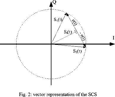
Where a(t) and 0(t) are time varying magnitude and phase respectively. This signal is split into two constant envelop signals after SCS block.

S i (t) = 2[S_t(t)-e(t)]                 (2)

S 2 (O^^^^^ + e^)]             (3)

According to (4), e(t) is perpendicular to S t (t) and from (1) to (4) the magnitude of S_i(t) and S₂(t) are equal to ^. According to Fig.2 these signals have constant magnitude and variable phase which changes by the input signal level.

The power amplifier in each path is characterized using a nonlinear memoryless model which depends on the level of the input signal. The accuracy of the model was shown in some previous works [12], [13] and [14]. The complex gain of the amplifier is extracted from measurements of AM–AM and AM–PM conversions of a Mitsubishi M68749 amplifier (with a driver) at 390 MHz (50 system) [12]. The amplifier is modeled as follows:

G_n (|v(t)|) = M „ (Ht)|)

• e^ n ⁽ l ^y(£) l)                n          (5)

= 1,2

Where e(t) is defined as:

eK^-tour1       <4>

Where Gn(|v( t)|) is a complex model of the power amplifier gain and Mn(|v(t)|) and 0n(|v(t)|) are variable magnitudes and phase which changes with the input signal level as follows:

М п (| v( t)|) =200+800|v(t)|

- 12760| v (t)| ² + 67930| v (t)| ³

- 193540| v( t)| ⁴ + 281970|v( t )|⁵ - 162240|v( t )|⁶

0 „ (|v( t )|) = 1.1426 + 2.2584| v ( t )| - 27.676| v ( t)| ² + 147.2407|v( t )|³ - 461.0754|v( t )|⁴ + 722.6528|v( t )|⁵ - 432.1345|v( t )|⁶

should be added in the LINC architecture to measure the error signal and modify complex coefficients in each path adaptively. In the next section MGA is introduced briefly.

• III.    Modified Gradient Algorithm

Optimization problems naturally arise from applications such as signal processing, data analysis, network design and etc. Among many applications error signal optimization (minimization) has attracted so much attention. The general form of optimization problem can be written as (15).

min(max) f(X)      X ∈ R "             (15)

As a result, the amplifier output signal can be shown as follows:

Sol (t)=vi (t). Gi(|vi (t)|)(8)

So2 (t)=v2 (t). G2 (|v2 (t)|)(9)

Where v i ( t ) and v 2 ( t ) are input signal of the power amplifiers PA_i and PA 2 . Assuming ideal digital to analog converters the following relations are valid.

vi (t)=Si (t)(10)

v2 (t)=S2 (t)(11)

As a result the output signal will be obtained according to(8) and (9) as follows:

S o (t)= v i ( t ). G i (| v i ( t)|)

+ v 2 ( t ). G 2 (| v 2 ( t )|)

With substituting (10) and (11) in (12), S_o (t) will be calculated as follows:

S o (t)= S i (t). G i (| v i (t)|)

+ S 2 (t). G 2 (| v 2 (t)|)

If G i (| v_i (t)|)=G 2 (| v₂ (t)|) , then the output signal will be an integer multiple of the input signal. With substituting (2) and (3) in (13) the general form of the input signal will be calculated as follows.

S o (t)

G i (| v i ⁽ t)|)+ G 2 (| v 2 ⁽ t)|)

= ^St ^{( t )}              2                         (14)

G i (| v i (t)|)-' G 2 (| v 2 (t)|)

-e ⁽ t )-------------о-------------

The second term in (14) is considered as an error signal. This term should be tend to zero for having higher spectrum efficiency. Therefore a feedback path

One of the simplest and most efficient methods to solve the above equation is gradient method which is proposed by Cauchy in [15]. In this method the value of x is calculated by a following recursive relation:

^Xk+i = ^Xk - ^ k 9 k

Where 9 k = ∇ f( X k ) is the gradient of f(X) for X — X k . Obviously this method is useful when the gradient of f(X) is available and isn’t complicated to obtain. Also ^ak is a coefficient that determines convergence speed. The larger the value of this coefficient the faster the convergence speed. It should be noted that if this coefficient be so large then the system will be unstable. In [11] this coefficient is considered as a constant factor. As a result the algorithm experiences a constant evolutionary path to reach the optimum solution.

Gradient algorithm has some drawbacks ([16], [17]) such as low convergence speed. ^ak in (16) can be considered as a variable value depending on the instantaneous gradient value. In this situation f(X) convergence can be expedited. So the conventional gradient algorithm can be modified with a variable coefficient that changes with instantaneous gradient and x values. Barzilai and Borwein (BB) proposed one of the most efficient modified gradient methods, namely BB gradient method or two-point stepsize gradient method [18]. In the BB gradient method, the stepsize a_k is derived from a two-point approximation of the secant equation [19]. Finally modified ^ak is obtained as follows:

« k =

Where Sk-i  Xk - Xk-i and Ук-1 =   - 3k-l . So the recursive relation for x in MGA is as:

r         Sk-lSk-1 к xk+l =  - cT—-— I 9k

Vk-Wk-lJ

With these changes convergence process will not be linear, thus the performance of the conventional gradient method will be improved. In next section a feedback path will be added in the conventional LINC structure to minimize the effect of gain and phase unbalances.

• IV.    Reduction of Nonlinear Effect  in  LINC

Transmitters

Although, the LINC technique is used to increase both efficiency and linearity of power amplifier but the efficiency of this method decrease with amplitude and phase mismatches between two signal paths ([20]-[22]). These mismatches come from unbalanced power amplifiers and other factors like manufacturing process. Thus a method is provided to modify the conventional LINC structure in a way to reduce the gain and phase errors and calibrate two branches. According to this method, two complex coefficients are applied in each path as a signal gain to minimize the error that rise from mismatches (Fig.3). The MGA is used for error minimization that changes the values of K( and K2 adaptively. K( and Kh have complex values so they can affect on both magnitude and phase of the signal.

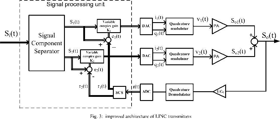
For error recognition a reference signal is required to modify K₍ and K₂ accordingly. For this purpose the outputsignal is divided by G _L and after passing through the quadrature demodulator and analog to digital converter, two reference signals, r₍(t) and r₂(t) are obtained. So S₁ (t) — ( ( (t) and S₂ (t) — r₂ (t) show the amount of error signal in top and bottom branches. If two branches are matched exactly then the error signal will be zero and the output signal will be linearly amplified. But if two branches have some imbalances then the value of the error signal will be nonzero and the output signal will have distortion. In Fig.3 nonlinear effects appear after power amplifier blocks. From Fig.3, r(t) is calculated as follows:

So (0

r(t) = r ( (t)+r 2 (t)=-^ (19)

G_l in the above equation is equivalent to the approximation of loop gain. If this approximation not be precisely correct, then a small amount of error will remain in the output that will absorb in K₍ and K₂ coefficients. According to (12) and considering that K₍ and K₂ are multiplied in the gain of each path, the following equation will be obtained.

r(t)

= -((t). K. G((| V( (t)|) + -2 (t). K2. G 2 (| V2 (01(20)

Gl

Similar to (1),r(t) can be written in complex form as follows:

r(t)=0(t)eMt)    0

Like (2) and (3), r( (t) and r2(t) will be calculated as:

Г((О = 2 [r(O — er(O]

Г to = 2 [r(0 + erto]

er(t) will be obtained like (4) as:

eXO=MoJ5|)—1

According to Fig.3. e( (t) and e2 (t) will be computed as:

61 ( t )= Si ( t )- T1 ( t )

e₂ ( t )= S₂ ( t )- r₂ ( t )                  (26)

V_KJn ≈-2en(t)∙(r^(t))^∗   n=1,2       (33)

The target function for optimization is considered as:

jn = E[|en (t) ²|]      n=1,2            (27)

where E[∙]denotes the statistical expectation operator. The above equation can be simplified as follows:

Here the target function is /( ^1 ) and /( ^2), similar to function f ( X ) in (15). According to MGA that has mentioned in previous section, and (18) the recursive relation for K^ and ^^2 will be computed as:

Ki ( m +1)= Ki ( m )

-(           ) Vj_K1 ( m )     (34)

jn =E[en(t). en(t)^∗]

= E[(Sn(t)-rn(t)).(Sn(t)-rn(t))∗]

= E[|S n (t) 2|+|r n (t) 2|-Sn(t). rn(t)∗

-Sn(t)∗rn (t)]

n=1,2

K₂ ( m +1)= K₂ ( m )

(

S^T ) ^VJk₂ ⁽ m ⁾

The gradient of the objective function is computed by means of partial derivatives and will be obtained as follows:

=

=    +

n=1,2

Where K_n = + jKi_n . That Kr_n and Ki_n are real and imaginary part of K_n .According to Fig.3. rn (t) can be considered as:

Where S-m-1 = ( m )- Ki ( m -1) , ⁼ ^2 ⁽ m )- K₂ ⁽ m -1) , Ут-1₁ = ( m )^- Vj_K1 (m-1) and Ут-1₂ = ( m )^{- V}Jk₂ (m-1) ^. ^1 and K₂ are changed in a way to minimize e and e 2 . So here ^1 and ^2 will be reached to theirs steady state much faster than conventional gradient algorithm. When e and e 2 tend to zero, •Si ( t ) will be equal to 7*1 ( t ) and 1S2 ( t ) will be equal to ^*2 ( t ) exactly. As a result distortion in the output signal will be decreased greatly. In the next section simulation results have been performed to validate the mentioned predictions

S n (t) ^n^n ^rn(t)=— г---

UL

n=1,2         (30)

Finally the gradient of (27) will be computed as:

^KnJn

-2 E

*|S " (t) ² |( - | ^| ; | ^| -

Ik 2I^{9 |} Gn | |K ⁿ_| ак_п ^∗

+_| Gl |     ^-

n=1,2

Considering that The partial derivative terms of the G_n respect to the variable К_л are very close to zero in the working region of the amplifier and using (25), (26) and (30), (31) will be simplified as:

и ≈-2 E(e - (t) ∙(^r 7 (t)) ∗ )

n=1,2

With instantaneous approximation of the expectation value, the following relation will be obtained.

V. Simulations and Results

In this section the input signal is a differential quaternary phase-shift keying modulated signal filtered with a squared-root raised cosine with a 0.35 rolloff factor at 36 Kbps which has the same characteristic with terrestrial trunked radio (TETRA) signal. TETRA is an open standard developed by the European Telecommunications Standards Institute (ETSI). The main purpose of the TETRA standard was to define a series of open interfaces, as well as services and facilities, in sufficient detail to enable independent manufacturers to develop infrastructure and terminal products that would fully interoperate with each other's. TETRA has four user channels on one radio carrier and 25 kHz spacing between carriers. One of the main disadvantages of TETRA is that it requires a linear power amplifier to meet the stringent RF specifications that allow it to exist alongside other radio services. Therefore the spurious emission in the first adjacent channel must be less than -60dBc. The carrier frequency is equal to 390MHz. it should be mentioned that sampling rate is chosen 2.3 MHz which is 128 times the sampling rate of TETRA signal. In fact we considered a signal with much higher PARR (peak to average ratio) than TETRA. A sampling rate too high supposes that all digital blocks in the DSP, mainly the signal component separator, must run at a much higher rate than without a

correction method, and the ADC and DACs must be much faster. More information about the sampling rate in a LINC transmitter can be obtained in [23].

To demonstrate the mismatches between two paths, several variations had been applied in some coefficients of the gain and phase polynomial.

Fig.4 shows the power spectrum density of the input signal and normalized output signal with some unbalances in amplitude and phase in two branches. According to Fig.4 small amount of phase and gain mismatches, increase ACI significantly. As a result this make it inapplicable to use LINC technique in practical systems. Therefore it is necessary to modify the output spectrum and minimize the error signal.

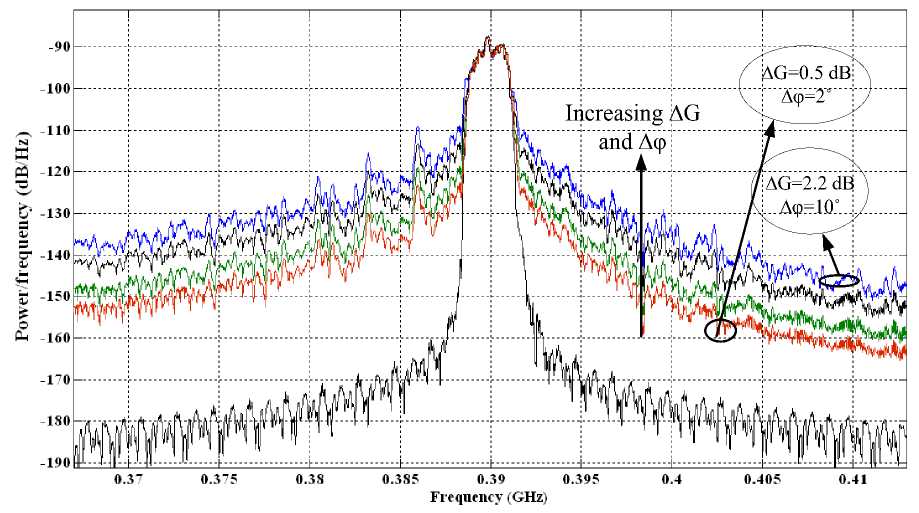
Fig. 4: input and normalized output power spectrum density

First channel second channel third channelfourth channel

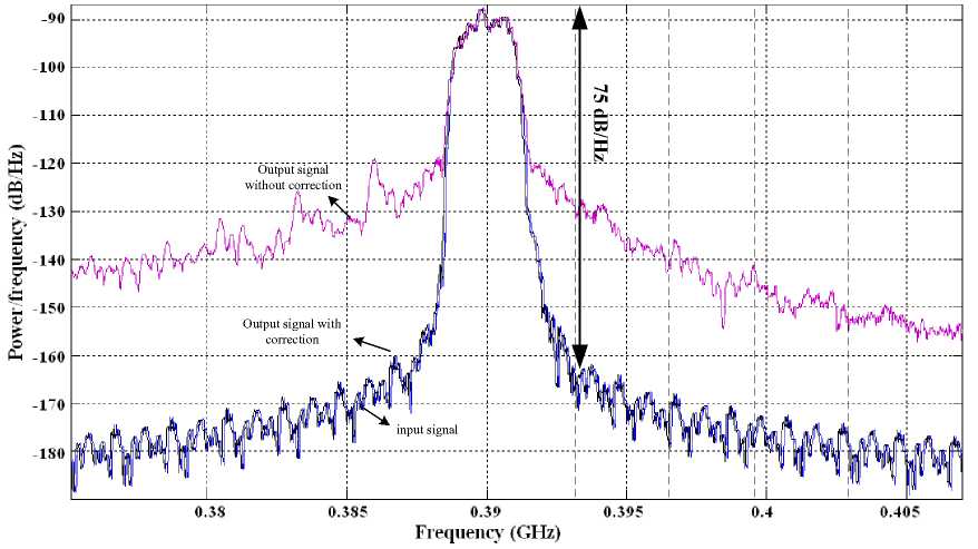
Fig. 5: input and normalized output power spectrum density

In fig.5 power spectrum density of the input signal and output signal with and without correction method is demonstrated. The output signal in this case has gain imbalances around 0.8 dB and phase imbalances about

3 ° between two branches of the signal path. High efficiency spectrum is obtained using adaptive MGA. Also ACI is decreased significantly (approximately -40 dB/Hz) and make it possible to use in TETRA standard.

One of the main advantages of this work over other similar works is its lower ACI and fast convergence speed. Fig.6 compares the ACI of the proposed MGA with conventional gradient algorithm which was investigated by [11]. Considering Fig.6 the output signal corrected with MGA has lower distortion in all channels compared with gradient algorithm.

First channel second channel third channel fourth channel

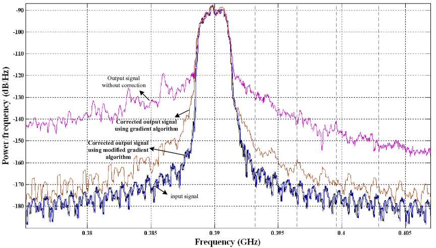
Fig. 6: input and normalized output power spectrum density

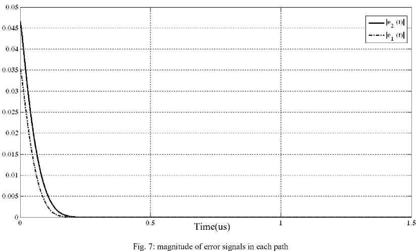
The evolution of error signals, e1 (t) and e2 (t), are pictured in Fig.7. MGA has little transient time (approximately 0.2 us) compared with conventional gradient algorithm (about 1.5 us). This convergence time is suitable to be implemented in real system.

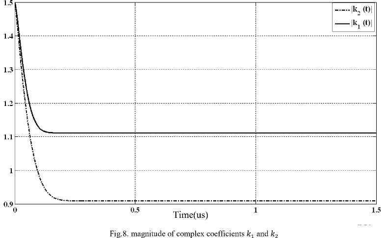
Magnitudes of Кг and K2 are shown in Fig.8 for phase imbalances of 10° and gain imbalances of 1.5 dB between two branches. This coefficients change in a way to minimize the error signals.

EVM=√(R2 +M2) - 2RMcosα n=1,2 (40)

where R is the magnitude of ideal vector, M is the magnitude of measured vector and α is the phase error between them. In digital communications, EVM should be less than a certain value. In the proposed structure EVM for some small imbalances between two branches, without correction method is about 9% .While this value is reduced to 1% after applying correction method.

• VI. Conclusion

All digital self calibrating LINC transmitters using an adaptive MGA has been described. Using this method major limitations of the LINC technique will be resolved. This architecture uses MGA to change the value of complex coefficients ^1 and ^2 , which is known as path gain in a way to reduce the adjacent channel interference and make it applicable to use in TETRA standard. this method could be implemented in a real system by means a suitably powerful DSP device. The main advantages of this algorithm over other algorithms are fast convergence time (around 0.2 us) and lower interferences in adjacent channels compared with similar works.