Mobile Robot Path Planning with Randomly Moving Obstacles and Goal

Published Online March 2012 in MECS

Mobile robots are automated machines that are capable of movements in a given environment [1]. Usually, these autonomous mobile robots are used in higher, deeper, riskier environments where humans cannot imagine treading [2]. In order to achieve tasks, they are intelligent in deciding their own actions. Especially, in an environment with obstacles, it is necessary to plan a collision-free path for the mobile robot to reduce cost, energy, time, and distance [1].

Mobile robots were first installed in factories around 1968 and were mainly automated guided vehicles (AGVs) and vehicle transporting tools following a predefined trajectory. However, the study in this area deals now with autonomous indoor and outdoor navigation. Autonomous mobile robots execute the task in four stages: perception of the environment, self-localization, motion planning, and motion generation [2].

In structured environments, the perception process allows maps or models of the world to be generated that are used for mobile robot localization and motion planning. In unstructured environments, however, the mobile robot has to learn how to navigate. The localization process allows a mobile robot to know where it is at any moment relative to its environment. For this purpose, sensors are used that will take measurements of the mobile robot’s current state and its environment [2]. In motion planning, the path to be taken is decided and in motion generation, the planned motion is implemented and monitored [3].

A great number of different techniques have been and are being developed in order to carry out efficient mobile robot obstacle avoidance, while the obstacle avoidance algorith m determines a suitable direction of motion based on recent sensor data. Obstacle avoidance is performed locally in order to ensure that real-time constraints are satisfied [4]. A fast update rate of the obstacle avoidance is required to allow the mobile robot to move safely at high speeds.

The potential field method is commonly used for autonomous mobile robot navigations because of its simple and elegant mathematical analysis. The basic concept of the potential field method is to fill the mobile robot’s workspace with an artificial potential field where the mobile robot is pulled to its goal and is pushed back from the obstacles [5]. However, substantial shortcomings that are inherent to these principles do exist and are presented in [6].

Borenstein and Koren [7] developed the Virtual Force Field approach to detect unknown obstacles and simultaneously to steer the mobile robot towards the goal. This method combines the potential field method with a certainty grid. One problem inherent to this method is the possibility of the mobile robot getting trapped. Borenstein and Koren [8] developed the Vector Field Histogram (VFH) approach, a real-time obstacle avoidance method, for fast-running vehicles, which has a significant improvement over the Virtual Force Field approach. Brooks [9] achieved collision-free path planning by good representation of free space. 3-D collision-free path planning was achieved by Herman [10]. All these methods were developed by assuming that both the obstacles and the goal are stationary. In many real-life implementations, however, everything is dynamic. Not only the obstacles, but also the goal is moving.

Fujimura and Samet [11] presented a method for path planning among moving obstacles, where time is included as one of the dimensions of the model world. Thus, the moving obstacles are regarded as stationary in the extended world. The major problem in this approach is that the information of the obstacle is provided a priori to the mobile robot. Chakravarthy and Ghose [12] presented a collision-cone approach for collision detection and navigation based on kinematic equations. The collision conditions are established based on the range and line-of-sight rates. Ge and Cui [13] presented a dynamic potential field method to avoid randomly moving obstacles and to reach a randomly moving goal. However, there are some problems, for example, local minima and free-path local minima. Berg and Overmars [14] extended a classical probabilistic road map method, which was originally designed for static environments, to the dynamic environment. This method has limited performance when obstacles are allowed to move in the environment.

Recently, Seder and Petrovic [15] presented a dynamic window method. This approach works well in static environments and do not perform well in dynamic environments due to the large difference in the collision detection and the necessity to control the speed of the mobile robot for the two different environments, dynamic or static. Masehian and Katebi [16] presented a new sensor-based online method for path planning of mobile robots with a moving goal among stationary and moving obstacles. Belkhouche [17] introduced the concept of the virtual plane for path planning in dynamic environments. The virtual plane is an invertible transformation equivalent to the workspace, which is constructed by using a local observer.

In this study, dynamic path planning for a mobile robot that can track and reach a randomly moving goal is generated, while multiple randomly moving obstacles of various shapes and sizes are avoided. Here, “random” means that the trajectories of the moving obstacles and goal are not known a priori . The MATLAB 3-D simulations mimic closely the real-life environments.

In Section 2, advantages of the proposed method are presented compared to the dynamic potential field method. The concepts of the new mathematical approach are discussed and the related equations are derived. Special cases are also discussed in this section. In Section 3, simulation results for the multiple randomly moving obstacles and the randomly moving goal as well as the tracking path of the mobile robot are presented. Section 4 gives the conclusion and future work.

• II.    DEVELOPMENT OF THE SCHEME

The main object of the developed scheme is to propose a new method based on 3-D geometry for a mobile robot to track and reach a randomly moving goal in a 3-D environment with avoidance of multiple randomly moving obstacles, while no knowledge of the movements of the goal as well as the obstacles is known to the mobile robot a priori .

• A.    Superior to the dynamic potential field method

Ge and Cui [13] proposed a new potential field method for path planning of a mobile robot in a dynamic environment where both the obstacle and the goal are moving. According to this method, the attractive potential is a function of the relative position and velocity of the goal with respect to the mobile robot, and the repulsive potential is defined as the relative position and velocity of the mobile robot with respect to the obstacles. Thus, the virtual force is defined as the negative gradient of the potential in terms of the position and velocity rather than the position only. They discussed two problems when this method is applied to dynamic environments.

(1)Local minimum

Consider the case that the mobile robot, the obstacle and the goal are moving in the same direction along a line and the obstacle is in between the mobile robot and the goal as shown in Figure 2.1. According to the dynamic potential field method, the mobile robot is always repelled from the obstacle and cannot reach the goal. This is called the local minimum problem. To solve this problem, Ge and Cui [13] suggested that the mobile robot needs to wait until either the goal or the obstacle changes its position. After a certain time of waiting, if the mobile robot is still in the same situation, the conventional local minimum recovery approaches such as the wallfollowing method proposed by Yun and Tan [18] are applied. In their method, the mobile robot follows the current obstacle contour, which is the boundary of the obstacle that pushes the mobile robot away. Once the mobile robot is recovered from the trapping situation, it will follow the original method to reach the goal.

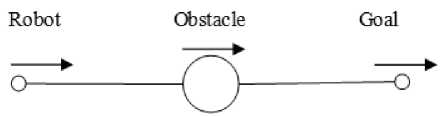
Figure 2.1 Local minimum

(2)Free-path local minimum

Another kind of local minimum problem is generated when the goal is within the influence range of the obstacle. Consider the case that both the mobile robot and the goal are near to the obstacle, with the goal in between the mobile robot and the obstacle, moving along a line as shown in Figure 2.2. In this case, when the mobile robot tries to reach the goal, it is repelled from the obstacle at the same time. The mobile robot can reach the goal only if the velocity of the mobile robot is large enough. This is called the free-path local minimum problem. This problem is solved by setting the repulsive force to zero, i.e., only the attractive force is taken into account [13].

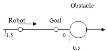
Figure 2.2 Free-path local minimum

The developed scheme eliminates the problems of the dynamic potential field method.

• (1)    The local minimu m problem as well as the free-path local minimum problem is avoided by moving the mobile robot through the via-point to reach the goal, even though all the aforementioned three bodies are moving along a line with the same direction.

(2)The collision with any obstacle is detected long before the collision could take place. Therefore, the chance for any collision is well prevented.

• (3)    The safety zone of the obstacle, which is to be defined in Subsection B, can be varied depending upon requirements.

• B.    Collision detection

The convention used in this study relates to analytic geometry and 3-D vectors.

(1)Mobile robot

The mobile robot is defined as a point object R ( R , R , R ) in the 3-D space. It is represented as a solid dot in MATLAB plots.

(2)Obstacle

Obstacles are unpredictable objects that the mobile robot may encounter during the execution of the task. In general, obstacles can be of any shape and size with a volume characteristic. Each obstacle’s position is represented by C(C ,C ,C ) . Here, the obstacles are in random movements. The mobile robot has to be alert at all times to avoid randomly moving obstacles and, at the same time, to move towards a randomly moving goal.

• (3)    Safety zone

The safety zone of the obstacle is the region around the obstacle that the mobile robot must avoid. It is a sphere with radius r around the obstacle as shown in Figure 2.3. The radius r is chosen in accordance with the size of the obstacle. If the obstacle is of an irregular shape, radius r is one half of the longest side of the obstacle. The sphere drawn by using this longest side should “wrap” the entire obstacle.

(4)Goal

The goal is defined as a point object G ( G_x , G_y , G_z ) in the 3-D space. It is represented as a square in MATLAB plots. The goal moves randomly.

In general, the obstacles are detected by sensors, which are assumed being mounted on the mobile robot. When the mobile robot detects the presence of any obstacle with the help of the sensors, it has to decide whether the obstacle is in its way. The steps below are taken to detect any possible collision with an obstacle.

The equation of a line passing through two points, the mobile robot’s current position R(Rx,Ry,Rz) and the goal’s current position G(Gx,Gy,Gz) , is x - Rx __ y - Ry __ z - Rz

--------—--------—-------— A               (2.1)

Gx - Rx  Gy - R   Gz - R xx yy zz where X is a constant.

Robot Travel Path

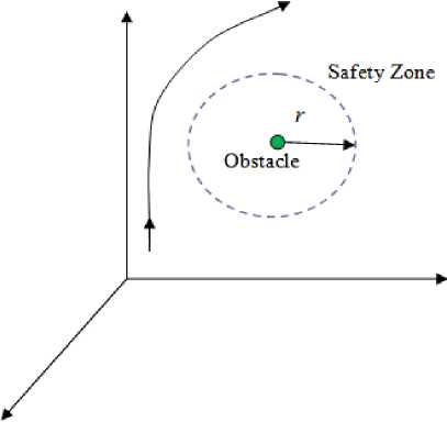
Figure 2.3 Safety zone of the obstacle

The equation of a sphere that has the center c ( C _x , C _y , C _z ) and radius r representing the safety zone of the obstacle is

( x - C x )² + ( y - C y )² + ( z - C z )² — r ²             (2.2)

Combining (2.1) and (2.2) results in

[ A ( G x - R x ) + ( R x - C x )]² + [ A ( G y - R y ) + ( R y - C y )]² + [ A ( G z - R z ) + ( R z - C z )]² — r ²

(2.3)

The line and the sphere may intersect in three possibilities:

(1)No intersection

(2)Intersection at only one point

• (3)    Intersection at two points

Mathematically, if the quadratic equation (2.3) has no real solution, then the line and the sphere do not intersect (Case (1)). If this equation has only one real solution, then the line intersects the sphere at only one point, i.e., the line is a tangent line to the sphere (Case (2)). If this equation has two real solutions, then the line intersects the sphere at two points (Case (3)).

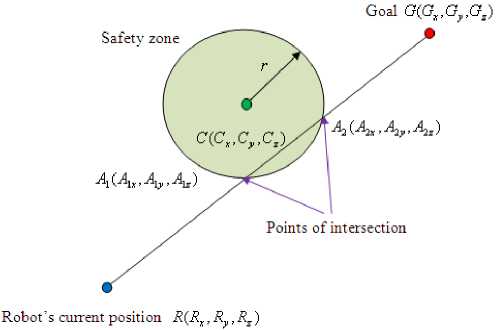
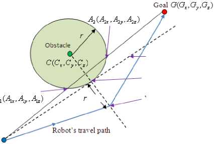
For Case (1) and Case (2), the mobile robot does not hit the obstacle, and it moves towards the goal without any collision. For Case (3) as shown in Figure 2.4, there is a collision, since the obstacle is in the way of the mobile robot to its goal. To avoid the collision, a feasible path between the current mobile robot position and the goal position needs to be decided. In this study, the path is generated by locating a via-point with the use of the proposed mathematical approach.

Robot's current position

MR«.R,,R^

Figure 2.4 Intersection of the line and sphere (Case 3)

A

Tangent line

Tangent point T(T_X, T_y ,T_X)

Via-point ^,^7,)

Figure 2.5 Mobile robot’s path through the via-point

• C.    Mathematical approach to locating the via-point

A novel mathematical approach is proposed to generate the path of the mobile robot in a 3-D environment to reach a randomly moving goal with avoidance of randomly moving obstacles. The key of the mathematical approach involves locating the via-point that is to be aimed at so as to avoid the possible collision with any randomly moving obstacle by using 3-D geometry of spheres and planes. After locating the viapoint, the mobile robot moves to the via-point and takes its position as the current position for the next movement.

The via-point V(Vx ,Vy ,Vz) is a point on the line drawn from the obstacle’s center C(C ,C ,C ) to a xyz unique tangent point T(Tx ,Ty,Tz) of the sphere and is at a distance of a radius r from the unique tangent point. The unique tangent point T(Tx ,Ty,Tz) is one of the intersection points of the tangent lines drawn to the sphere from the mobile robot’s current position R(Rx,Ry,Rz) . In order to locate the via-point V(Vx,Vy ,Vz)   , the unique tangent point

T ( T_x , T_y , T_z ) needs to be decided first. See Figure 2.5. The steps below are involved to locate the via-point V ( V x , V y , V z ) .

• (1)    The tangent point T ( T_x , T_y , T_z ) on the sphere

The tangent point T ( T_x , T_y , T_z ) is a point on the surface of the sphere. Therefore, the equation of the sphere passing through the tangent point T ( T_x , T_y , T_z ) with its center at C ( C , C , C ) and radius r is xyz

• (2)    The tangent plane of the sphere at the tangent point T ( T x , T y , T z )

The equation of the tangent plane to a surface defined by an implicit equation f (x, y, z) = 0 at the point T(Tx,Ty ,Tz) is f (x - T ) + f (y - T ) + f (z - Tz ) = 0 xyz dx         dy          dz

Since the surface here is a sphere described by (2.2),

Thus, f = 2( x - Cx) x dx

^ = 2( У - Cy) oy f = 2( z - Cz)

d z

(2.5)

(2.6)

(2.7)

Since T ( T_x , T_y , T_z ) is a point on the surface of the sphere, the equation of the tangent plane becomes

^{2( T} x ^{- C} x ^{)( x -} T x ) ^{+ 2( T} y ^{- C} y ^{)( y -} T y ) + 2( T z - C z )( z - T z ) = 0

(2.8)

Simplifying the tangent plane equation (2.8) by using (2.4) leads to

( T x - C x )² + ( T y - C y )² + ( T z - C z ) 2 = r r-

(2.4)

2 x(T x - C x ) + 2 y(T y - C y ) + 2 z ( T z - C z )

- T x ² - T y ² - T z ² + C x ² + C y ² + C z ² - r ² = 0

Furthermore, the tangent plane of the sphere at the point T ( T_x , T_y , T_z ) that also passes through the external point R ( R , R , R ) is then of the form xyz

2 R (T_x - C_x ) + 2 R_v (T_v - C_v ) + 2 R_z (T_z - C_z ) xx  x   yy  y   zz  z

- T x ² - T y ² - T z ² + C x ² + C y ² + C z ² - r ² = 0

(2.10)

These equations can be solved by using the Cramer’s Rule.

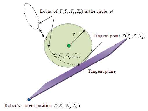
It should be noted that this tangent plane is drawn at an arbitrary tangent point and is not unique. The locus of the tangent planes passing through R ( R_x , R_y , R_z ) on the sphere is actually a circle along the circumference of the sphere and is defined as circle M . Figure 2.6 shows one of the tangent planes and the circle M .

	A 1 x	A 1 y	A 1 z
K =	R x	R y	R z	(2.13)
	C x	Cy	C z

D

M = — к

Figure 2.6 One of the tangent planes and the circle M

If K is nonzero (for the planes not passing through the origin of the sphere), the coefficients L , M and N are obtained as follows.

^{1   A} 1 y    ^A 1 z

L = D 1   R_v  R_z

K  yz

1   C y   C z

(2.14)

A 1 x R x C x

1   A 1 z

1   R z

1   C z

A1x   A1y

N = DR  R1

Kxy

C   C1

xy

(2.15)

(2.16)

(3) The plane П passing through three points A ₁( A _{1 x} , A _{1 y} , A _{1 z} ) , R ( R_x , R_y , R_z ) and C ( C x , C y , C z )

The plane П passing through three points A ₁( A _{1 x} , A _{1 y} , A _{1 z} ) , R ( R_x , R_y , R_z ) and C ( C_x , C_y , C_z ) can be defined as all the points ( x , y , z ) that satisfy the determinant equations below.

These equations are paramet ric in D . By co mparing (2. 11) and (2. 12), and using (2.13), D is identified as K . Therefore, the equation of the plane П passing through three points can be obtained as

Where

(2.17)

x - A 1 x	y - A 1 y	z - A 1 z
Rx - A 1 x	Ry - A 1 y	Rz - A 1 z
Cx - A 1 x	C y - A 1 y	C z - A 1 z
x - A 1 x	y - A 1 y	z - A 1 z
= x - Rx	y - Ry	z - Rz =(
x - C x	У - C y	z - C z

(2.11)

The plane П can also be described as an equation in the form of Lx + My + Nz - D = 0 by solving the set of equations below.

LA 1 _x + MA 1 _y + NA 1 _z - D = 0

LR + MR_V + NR_Z - D = 0 xyz

LC_X + MC_V + NC_Z - D = 0 xyz

(2.12)

L = ( R y C z - R z C y ) - ( Ai y C z - Ai z C y ) + ( Ai y R z - A^R y ) M = ( R z C x - R x C z ) + ( A x C z - A z C x ) + ( A z R x - A x R z ) N = ( R x C y - R y C x ) - ( A x C y - A y C x ) + ( A i x R y - A i y R x ) ^D = ^A 1 x ^{( R}y ^Cz ^- R z C y ) ^{- R}x ^{( A} 1 y^Cz ^{- A} 1 z^Cy )

+ C x ( A 1 y R z - A 1 z R y )                          (2.18)

Thus, the equation of this plane П passing through the tangent point T ( T_x , T_y , T_z ) is

LT_x + MT_y + NT_z - D = 0 (2.19)

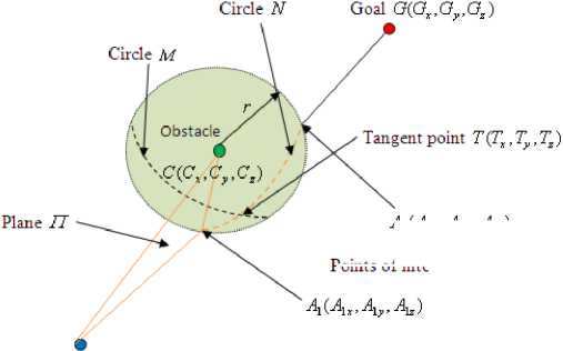
The intersection of this plane П and the sphere is also a circle along the circumference of the sphere and is defined as circle N . Figure 2.7 shows the intersection and the circle N . As well known, two circles along the circumference of a sphere have two intersections as long as the two planes where the circles are located are not parallel with each other. Thus, there presents a way to decide the unique tangent point.

T

x

Robot's current position R^R^.Ry.R^

Figure 2.7 Plane П and the circle N

^AA,A1

Points of intersection

(4) The unique tangent point

The three variables, T_x , T_y and T_z of the unique

tangent point can be decided by using three equations,

(2. 4), (2. 10) and (2. 19). They are rewritten

below for

convenience.

(T x — C x )² + (T y

C y )² + ( T z — C z )²

(2.4)

2 R x ( T x

C x ) + 2 R y (T y

C y ) + 2 R_z (T z

C z )

T x

T

y

T z

+ C_x

+ C y

+ C z

r ² = 0

(2.10)

— T y ( R y

C x

i.e., T_x =

where

C y ) — T z ( R z

C _y

C z

+ r

— T y ( R y

C_z ) + R_XC_X + R_VC_V + R_ZC_Z z   xx  yy  zz

( R x

^Cx ⁾

C y ) — T z ( R z

( R x

C x )

C z ) + k

(2.23)

k = R_XC_X + R_VC_V + R_ZC_Z xx  yy  zz

C x

C y

C

z

+ r ² , which is

a constant since all the variables at the right side of the

expression are known.

Substituting (2.23) into (2.19) results in

T y ( R y

C y ) — T z ( R z

C₂ ) + R_XC_X + R_VC _V + R_ZC_Z z   xx  yy  zz

L

C x

Cy

C z

+ r

( R x

C x )

LT + MTV xy

+ NT z

D = 0

(2.19)

Expanding (2.4) leads to

22 x ⁺ x

x x ¹ y ¹ y

2TyCy + Tz2 + Cz2

2TzCz = r

² x

² T_y

z     x ⁺ y ⁺  ^

z

r

2 T_xC_x

2Г C yy

2 T z C z

(2.20)

Expanding (2.10) leads to

2 R_xT_x

2 R_XC_X + 2 RT xx   yy

2 R_VC_V + 2 R_ZT_Z y y    zz

2 R_zC_z

т.

x

T.'

Ty

z + x

+ Cy

+ C z

r ² = 0

(2.21)

Substituting (2.20) into (2.21) results in

2 R_xT_x

2 R_XC_X + 2 RT xx   yy

2 R y C y + 2 R z T z

2 R z C z

+ C_x

+ C y

+ C z

r2

2 T_xC_x

2 T y C y

2 T z C z

+ C_x

+ C y

+ C z

r ² = 0

2 T_x ( R_x

C x ) + 2T y ( R y

C y ) + 2T z ( R z

C z )

2 R_xC_x

2 R y C y

2 R_zC_z + 2 C_x

+ 2 C y

+ 2 C z

2 r ² = 0

(2.22)

From (2.22), T_x can be expressed in terms of T_x , T y and

T_z as

+ MT_y + NT_z

— LT y ( R y

+ L [ R x C x

D = 0

(2.24)

C y ) — LT z ( R z

+ R y C y + R z C z

+ M T y ( R x

Thus,

T =T y z

+

C z )

C x

Cy

C z

+ r

]

C _x ) + NT z ( R.

L ( R z

M ( R x

D ( R x

C x

x

C x ) — D ( R x

C_x ) = 0

C z ) — N ( R x

^Cx ⁾

C_x ) — L ( R y

C y )

Cx) — L (RXCX + RVCV + RZCZ x    xx  yy  zz

Cy

C z

+ r ² )

M ( R x

C x ) — L ( R y

i.e., T y = T_zk 1 + k - 2

where

^k 1 =

^k 2 =

C y )

(2.25)

L ( R z — C z ) — N ( R_x

C ) x

M ( R_x — C x ) — L ( R y

D ( R x

C ' x

^C y ⁾

and

Cx) — L (RXCX + RVCV + RZCZ x    xx yy zz

C Cy

C z ² + r 2 )

M ( R x

C x ) — L ( R y

^Cy ⁾

Substituting (2.23) and (2.25) into (2.4) leads to

- C x

- T y ( R y - C y ) - T z ( R z - C z ) + k ( R x - C x )

(2.26)

+ ( T y - C y )² + ( T z - C z )² = r ²

T z ^{( - k} 1 R y ^{+ k} 1 C y ^- R z ⁺ C z ) ^{- k} 2 R y ^{+ k} 2 C y + k - C_xR_x + C x ²

+ [ ( T z k 1 + k 2 ) - C y ] ²( R x - C x )² + (T z - C z )²( R x - C x )²

= r ²( R x - C x )²

(T z k 3 + k 4 )² + [ ( T z k 1 + k 2 ) - C y ] 2 ( R x - C x ) 2

+ ( T z - C z )²( R x - C x )²

= r ²( R x - C x )²

k. = -LRV + kC -R7 + C7 and y  yzz where

Ra = -k^Rv + k^ Cv + k - CTRT + CT y     y      xx   x

T_z ² k ₃ ² + k ₄ ² + 2T_zk 3 k 4

+ [ ( T z k 1 + k 2 )² + C y ² - 2( T z k 1 + k 2 ) C y ]( R x - C x )²

+ T_z ² + C_z ² - 2T_zC_z J R_x - C_x )² = r ²( R_x - C_x )²

T_z ² k ₃ ² + k ₄ ² + 2 T_zk ₃ k ₄

+ T z ² k 1 ² + k 2 ² + 2 T z k 1 k 2 + C y ² - 2T z k 1 C y - 2 k 2 C y ]

( R x - C x )² + [ T z ² + C z ² - 2T z C z } R x - C x )² = r ²( R x - C x )²

T z ² [ k 3 ² + k 1 ² ( R x - C x ) ² + ( R x - C x ) ² ]

2 k 3 k 4 + 2 k 1 k 2 ( R x - C x ) ² - 2 k 1 C y ( R x - C x ) ²

⁺ T^z                   2

- 2 C_z ( R_x - C_x ) ²

⁺ к 42 ^{+[ k} 22 ⁺ C y ^{2 - 2} к 2 C y ⁺ C z ^{2 -} r ² j ^Rx ^- C x ^{) 2} = 0

(2.27)

Eq. (2.27) can be expressed in the form

AT_z ² + BT_z + C = 0

Where

A = ^k 32 ^{+ ( k} 12 ^{+ 1)( R}x ^- C x ) ² ,

B = 2 k ₃ k ₄ + [ 2 k 1 k ₂ - 2 k 1 C_y - 2 C_z ]( R_x - C_x ) ² and C = k ₄ ² + ^{[ k} 22 ⁺ C y ^{2 - 2 k} 2 C y ⁺ C z ^{2 -} r ² ]( ^Rx ^- C x ^{) 2}

Therefore, T_z

- B ± B b ² - 4 AC

2 A

(2.28)

As noticed, (2.28) gives two solutions of T_z .

Furthermore, as mentioned before, Ty can be obtained from (2.25), and Tx can be obtained by substituting Ty and Tz into (2.23).

Since (2.28) gives two solutions, two tangent points are therefore decided. However, only one of them needs to be selected to serve as the via-point. In this study, to reduce the moving time for the mobile robot, the tangent point nearest to the goal is selected. Suppose the two tangent points are T1(Tx1,Ty1,Tz1) and T2(Tx2,Ty2,Tz2), and the goal position is G(Gx, Gy , Gz) . Then the distance between T1(Tx1,Ty1,Tz1) and G(Gx,Gy,Gz) is

D 1 = V ( T x 1 - G x ) 2 + ( T y 1 - G y )² + ( T z 1 - G z )²

and the distance between   T ( T  , T , T ) and

G ( G x , G y , G z ) is

D 2 = V ( T x 2 - G x ) 2 + ( T y 2 - G y ) 2 + ( T z 2 - G z ) 2

If D ₁ is less than D ₂ , T ₁( T_{x 1}, T_{y 1}, T_{z 1}) is decided as the unique tangent point and otherwise T ₂( T_{x 2}, T_{y 2}, T_{z 2}) is.

(5) The via-point

The equation of a line passing through two points, the unique tangent point T(Tx ,Ty ,Tz ) and the obstacle’s center C(Cx,Cy,Cz) , is x - Tx  = y - Ty

Tx - Cx  Ty - Cy z - Tz Tz - Cz

= p

(2.29)

where в is a constant. (2.29) can be written as x = Tx + P(Tx - Cx ) y = Ty + e(Ty - Cy ) z = Tz + P(Tz - Cz )

(2.30)

By choosing different values of в , different points can be located on the line. The via-point is a point on this line, which is located at a distance of the radius r from the unique tangent point. That is, the via-point can be located by choosing в = 1. In other words, the coordinates of the via-point V ( V_x , V_y , V_z ) are obtained by

V x = T x + ( T x - C x )

V y = T y + ( T y - C y ) V z = T z + ( T z - C z )

(2.31)

Now, the via-point is located. Whenever the mobile robot detects a possible collision, the mobile robot aims at this via-point on its way to reach the goal.

• D.    Special cases

The mathematical approach presented in this study detects any possible collision and locates the via-point if any obstacle is in its way. However, there is a special case that the obstacle is coming from any other side towards the mobile robot’s current position as the example shown in Figure 2.8. In Figure 2.8, the mobile robot, goal and obstacle 3 are moving in the same direction, and obstacle 1 is moving towards the mobile robot’s current position. Obstacle 3 is located on the line created by the mobile robot’s current position and the goal. According to the mathematical approach, the mobile robot detects a possible collision with obstacle 3 and locates a via-point. Unfortunately, when the mobile robot is moving towards the via-point, obstacle 1 could be too close to the mobile robot or may have a collision with it.

To avoid this kind of collision, the mobile robot decides the distance between its current position and each obstacle every time. The distance between the mobile robot’s current position R ( R_x , R_y , R_z ) and the obstacle 1’s position C ₁( C_{x 1}, C_{y 1}, C_{z 1}) is

RC = V ( R x - C x i ) 2 + ( R y — C y i ) 2 + ( R z — C z 1 ) 2

(2.32)

Similarly, it decides RC ₂ , RC , RC ₄ and RC for each of the obstacles, respectively. If any of these distances is less than r + 0.05 (where r is the radius of the safety zone), the mobile robot is then going to move in the positive or negative direction of the unit movement vector of the obstacle in concern, which can be obtained from the current position and the previous position of the obstacle. In Figure 2.8, the current and previous position of obstacle 1 are C 1 ( C x 1 , C y 1 , C z 1 ) and C_{p 1}( C_{px 1}, C_{py 1}, C_{pz 1}) , respectively. The vector

C — C p1 is then,

C 1 — C p1 = ( C x 1 — C px1 , C y1 — C py1 , C z1 — C pz1 )    (2.33)

The unit vector of C — C p1 is therefore

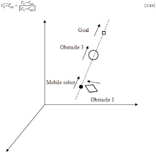
Figure 2.8 Special case 1

• (1)    The distance between R and C 1 is V(1.0- 3.0)² + (1.0- 2.5) 2 + (2.0 — 2.0)² = 2.5 <  r + 0.05 = 2.5 + 0.05 = 2.55. Thus, C₁ (3.0, 2.5, 2.0) is judged to be too close to the mobile robot or may have a collision with it.

• (2)    The next position of the mobile robot R_n , if moving in the positive direction of the unit movement vector (-1, 0, 0), would be (0.8, 1.0, 2.0). Then, the distance between R_n and C₁ would be 7(0.8- 3.0) 2 + (1.0- 2.5) 2 + (2.0 — 2.0)² = 2.66 >  r + 0.05 = 2.5 + 0.05 = 2.55. Thus, the mobile robot follows the direction (-1, 0, 0) to go to R n =(0.8, 1.0, 2.0).

• 2.    Suppose, at a certain instant, there are R (1.0, 1.0, 2.0), C 1 (3.0, 2.5, 2.0) and C p1 (2.9, 2.5, 2.0). Thus, the unit vector of ( C 1 – C p1 )=(1, 0, 0).

• (1)    The distance between R and C 1 is 7(1.0- 3.0)² + (1.0- 2.5) 2 + (2.0 — 2.0)² = 2.5 <  r + 0.05 = 2.5 + 0.05 = 2.55. Thus, C₁ (3.0, 2.5, 2.0) is judged to be too close to the mobile robot or may have a collision with it.

• (2)    The next position of the mobile robot R_n , if moving in the positive direction of the unit movement vector (1, 0, 0), would be (1.2, 1.0, 2.0). Then, the distance between R _n and C₁ would be 7(1.2-3.0)² + (1.0-2.5)² + (2.0 — 2.0)² = 2.34 <  r + 0.05 = 2.5 + 0.05 = 2.55. Thus, the mobile robot cannot follow the direction (1, 0, 0) to go to R_n =(1.2, 1.0, 2.0).

• (3)    The next position of the mobile robot R_n , if moving in the negative direction of the unit movement vector (1, 0, 0), would be (0.8, 1.0, 2.0). Then, the distance between R n and C 1 would be 7(0.8- 3.0) 2 + (1.0- 2.5) 2 + (2.0 — 2.0)² = 2.66 >  r + 0.05 = 2.5 + 0.05 = 2.55. Thus, the mobile robot follows the direction (1, 0, 0) to go to R_n =(0.8, 1.0, 2.0).

From the examples above, it is seen that, in this special case, it is absolutely depending on the current movement direction of the obstacle in concern for the mobile robot to decide whether to move in the positive or the negative direction of the unit movement vector of the obstacle.

To understand the above concepts better, numerical examples are presented.

1. Suppose, at a certain instant, there are R (1.0, 1.0, 2.0), C 1 (3.0, 2.5, 2.0) and C p1 (3.1, 2.5, 2.0). Thus, the unit vector of ( C 1 – C p1 )=(-1, 0, 0).

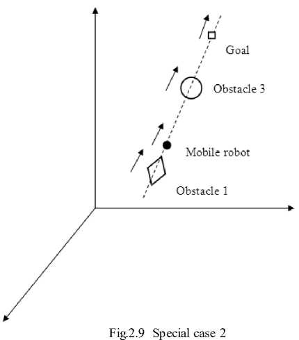
Another kind of special case arises when obstacle 1 is on the line created by the mobile robot and the goal and is also moving towards the mobile robot’s current position as shown in Figure 2.9.

According to the mathematical approach, the mobile robot locates a via-point only if the obstacle is in between the mobile robot and the goal. For the present case, the mobile robot locates the via-point to avoid obstacle 3 and moves towards that via-point. However, in the future, there is a chance of collision with obstacle 1, if it continuously moves on the same line and towards the mobile robot’s current position. This case is essentially the same as the special case before. The only specialty in this case is that the mobile robot detects a possible collision with obstacle 1 that is on the created line but not between the mobile and the goal. In Figure 2.9, if obstacle 1 is far away from the mobile robot’s current position though is on the created line, the mobile robot can ignore obstacle 1 and locates the via-point to avoid obstacle 3. If the distance between the mobile robot and obstacle 1 is less than r + 0.05, the mobile robot is to move in the positive or the negative direction of the unit movement vector of the obstacle 1 in the same way as shown in the special case before.

• (5)    Locate the via-point to avoid the closest obstacle in the way of the mobile robot and change the mobile robot’s direction of movement towards the via-point.

• (6)    Check for special cases. If there are special cases, go to step (7).

Else: go to step (8).

• (7)    Change the mobile robot’s direction of movement towards the positive or negative unit vector of the obstacle.

• (8)    Move the mobile robot along its direction of movement decided by (3), (5) or (7).

• (9)    If the goal is reached, go to (10).

Else: go to step (1).

• (10)    Stop.

The mobile robot finds its own current position and the current positions of the goal and obstacles from sensors. The mobile robot’s direction of movement is then defined towards the goal. The mobile robot creates a 3-D line of infinite length between itself and its goal. For the mobile robot, all the obstacles are in sphere shapes because of the defined safety zone for each obstacle. The intersections of the aforementioned line and the sphere are decided to detect the possible collision as explained in Subsection B. For a two point intersection, the mobile robot decides that there is going to be a collision and then locates a via-point. The mobile robot’s direction of movement is then changed towards the via-point. The mobile robot also checks for special cases in every iteration as explained in Subsection D. If there is going to be any special case, the mobile robot changes its direction of movement towards the positive or negative unit vector of the obstacle. Then, the mobile robot moves along its direction of movement in any one of the defined directions as shown in the flowchart depending upon the situation. If the mobile robot reaches the goal, the algorithm is stopped; otherwise, iterations will continue.

It is worth emphasizing that each time the goal position changes randomly, the mobile robot’s direction of movement also changes accordingly. Similarly, as an obstacle moves randomly, the mobile robot locates a new via-point in the present iteration and changes its direction of movement towards this new via-point. Figure 2.10 presents the flowchart for the mathematical approach to reaching the randomly moving goal while avoiding randomly moving obstacles.

• E. Algorithm and flowchart

The steps below give an idea of the algorithm used in this study. Each step is also explained in some detail.

• (1)    Start.

• (2)    Decide the new positions of mobile robot, goal, and obstacles (from sensors).

• (3)    Define the mobile robot’s direction of movement towards the goal.

• (4)    Check for any possible collision with obstacles in the near future. If a possible collision is detected, go to step (5).

Else: go to step (6).

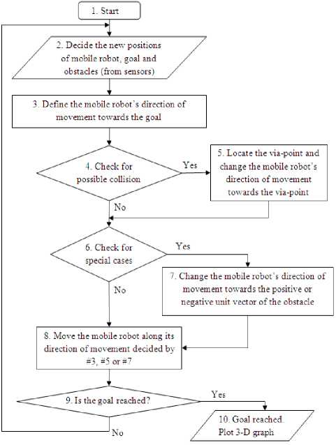
Figure 2.10 Flowchart for the mathematical approach

• III.    SIMULATION RESULTS

This section presents the simulation results. To represent 3-D graphs in two dimensions, the terms Azimuth (Az) and Elevation (El) are used. Azimuth (Az) is a polar angle in the x-y plane, with positive angles indicating counterclockwise rotation of the viewpoint. Elevation (El) is the angle above (positive angle) or below (negative angle) the x-y plane. Az and El are expressed in degrees throughout. Figure 3.1 illustrates Az and El in the 3-D coordinate system. The Az and El arrows indicate positive directions.

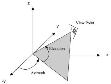
Figure 3.1 The Azimuth and Elevation

• (1) . Figure 3.2 gives the first set of simulation results, where the black solid dot represents the mobile robot, and the square represents the goal. The small solid dots represent the path traveled by the mobile robot, and the solid line represents the trail of the goal. The obstacles shown in this set of simulations are “wrapped” by invisible safety zones with a radius of 2.5 each. The “diamond”, “downward triangle”, “circle”, “plus” and “six-pointed star” stand for obstacles 1-5, respectively. In this study, the velocities of the goal and obstacles are taken as 0.1/iteration, and the velocity of the mobile robot is taken as 0.2/iteration.

In Figure 3.2(a), the initial positions of the mobile robot R (1,12,31), goal G (30,26,23), and five obstacles are shown. In Figure 3.2(b), the mobile robot is on its way to reach a randomly moving goal while all obstacles are also moving randomly. The mobile robot’s path and the trail of the goal can be seen. In Figure 3.2(c)-(d), the paths traveled by the mobile robot at the 110th iteration with different Az and El are seen. Figures 3.2(e)-(g) present the path traveled by the mobile robot at the 233th (final) iteration with different Az and El.

• (2) . Figure 3.3 gives the second set of simulation results. The obstacles shown in this set of simulations are “wrapped” by invisible safety zones with a radius of 4.5 each. In Figure 3.3(a), the initial positions of the mobile robot R (11,5,9), goal G (37,32,15), and five obstacles are shown. In Figure 3.3(b), the mobile robot is on its way to reach a randomly moving goal while all obstacles are also moving randomly. The mobile robot’s path and the trail of the goal can be seen. In Figure 3.3(c)-(d), the paths traveled by the mobile robot at the 140th iteration with different Az and El are seen. Figures 3.3(e)-(g) present the path traveled by the mobile robot at the 212th (final) iteration with different Az and El.

From Figure 3.3(e)-(g), it is clear that the mobile robot has reached the randomly moving goal successfully even though all the obstacles that have enlarged safety zones are moving randomly near the goal. For larger obstacles, safety zones are also enlarged so as to “wrap” the obstacle completely. It is seen then that the developed scheme works well even for large obstacles.

• (3) . Figure 3.4 gives the third set of simulation results. The obstacles shown in this set of simulations are “wrapped” by visible safety zones with a radius of 4.5 each. In Figure 3.4(a), the initial positions of the mobile robot R (11,5,9) , goal G (37,32,15) , and five obstacles that are the same as those in Figure 3.3(a) are shown. Also, it is seen that the goal is hidden under obstacle 4. In Figure 3.4(b), the mobile robot is on its way to reach a randomly moving goal while all obstacles are also moving randomly. The mobile robot’s path and the trail of the goal can be seen. It is seen again that the goal is still hidden under obstacle 4. In Figure 3.4(c)-(d), the paths traveled by the mobile robot at the 140th iteration with different Az and El are seen. Figures 3.4(e)-(g) present the path traveled by the mobile robot at the 212th (final) iteration with different Az and El.

As seen, in the generation of the path for the mobile robot, if the mobile robot detects any possible collision with any obstacle (say obstacle 5), it will locate the viapoint and move towards the via-point to avoid obstacle 5. In the next iteration, the mobile robot will still check for any possible collision with any obstacle again, since it is very possible that obstacle 5 is still in its way. The mobile robot will locate the new via-point at this time and move towards the new via-point to avoid obstacle 5. This is because of the change in obstacle 5’s position all the time, i.e., the random movement of obstacle 5. After a certain period of time, obstacle 5 may completely go away from the mobile robot’s path. It is very rare for the mobile robot to go to a via-point and then to the goal directly unless there are stationary or slowly moving obstacles. For a stationary or slowly moving obstacle, the path of the mobile robot is described as shown in Figure 2.5.

It should be noted that, in the generation of the path for the mobile robot, since all the bodies, i.e., the mobile robot, the goal as well as the multiple obstacles, are moving, it is difficult to catch by eyes whether any collision is occurring. To solve this problem, an alarm is set in MATLAB. As long as the mobile robot collides with any obstacle by any chance, the alarm will sound and the program will be stopped. Numerous real-time simulations with different settings are performed successively. Due to limitation of space, only three sets of simulation results are presented in this article,

• IV.    CONCLUSION

In this article, the proposed mathematical approach is implemented in real-time to generate a 3-D path for the mobile robot to track and reach a randomly moving goal while avoiding all five randomly moving obstacles. The developed scheme is effective with the drawbacks of the dynamic potential field method eliminated. The relative velocities of the mobile robot, goal, and obstacles are considered in the generation of the path. This method can be essentially implemented in real life to avoid randomly moving obstacles to reach a randomly moving goal. MATLAB simulation validates the proposed method.

Future work could be the consideration of a larger number of obstacles with different velocities. Moreover, multiple mobile robots can be considered in place of a single mobile robot.

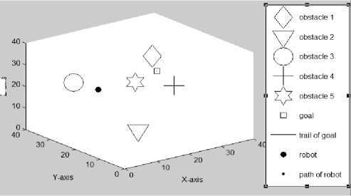
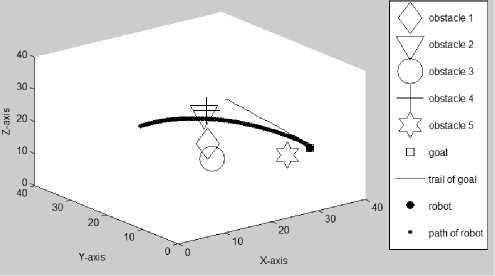
Figure 3.2(a) Initial positions of the mobile robot, goal, and five obstacles (Az=-38°, El =30°)

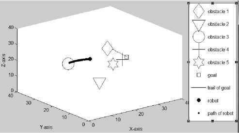
Figure 3.2(b) Path traveled by the mobile robot at the 70th iteration (Az=-38°, El =30е)

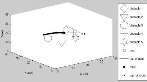
Figure 3.2(c) Path traveled by the mobile robot at the 110th iteration (Az=—38е, El=30°)

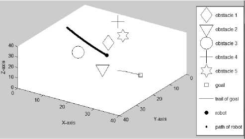
Figure 3.2(d) Path traveled by the mobile robot at the 110th iteration (Az=—34е, El =—50е)

Figure 3.2(e) Path traveled by the mobile robot at the 233th (final) iteration (Az=-38е, El=30е)

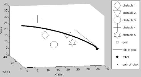
Figure 3.2(f) Path traveled by the mobile robot at the 233th (final) iteration (Az=-11°, El=14е)

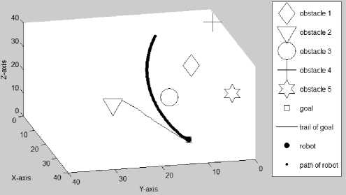
Figure 3.2(g) Path traveled by the mobile robot at the 233th ^7 ^7 О     О 1 U

(final) iteration (Az=—77 , El=32 )

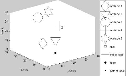
Figure 3.3(a) Initial positions of the mobile robot, goal, and five obstacles (Az=-38°, El=30е)

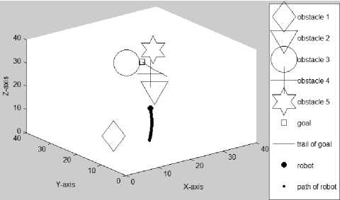
Figure 3.3(b) Path traveled by the mobile robot at the 87th iteration (Az=-38°, El=30е)

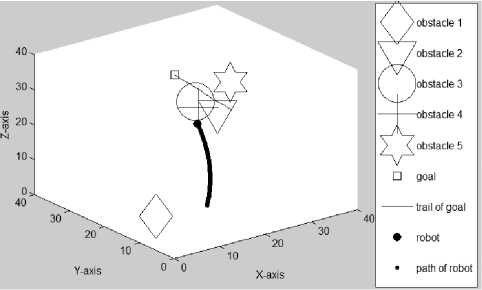
Figure 3.3(c) Path traveled by the mobile robot at the 140th iteration (Az=—38е, El=30°)

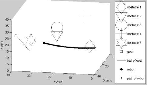
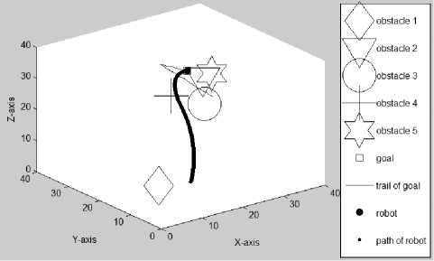
Figure 3.3(e) Path traveled by the mobile robot at the 212th (final) iteration (Az=-38°, El=30е)

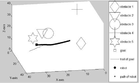
Figure 3.3(f) Path traveled by the mobile robot at the 212th (final) iteration (Az=-121°, El=26°)

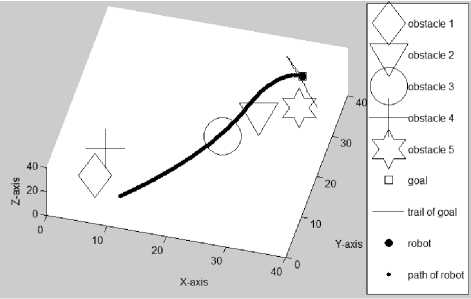
Figure 3.3(g) Path traveled by the mobile robot at the 212th л Г О 7 л О

(final) iteration (Az=15 , El=74 )

Figure 3.3(d) Path traveled by the mobile robot at the 140th iteration (Az=— 1U1 , El=—ZZ )

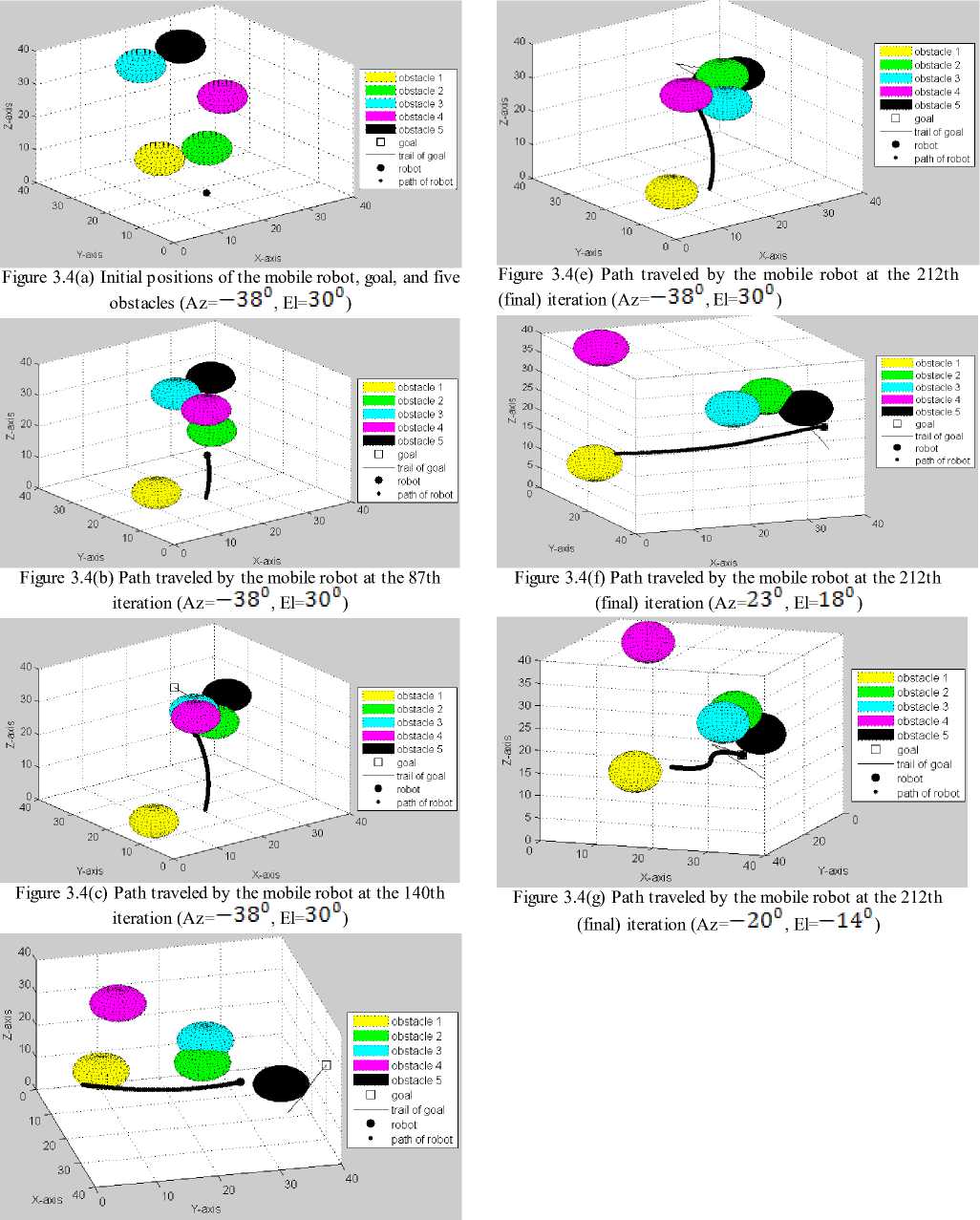
Figure 3.4(d) Path traveled by the mobile robot at the 140th iteration (Az= / / , El= о о)