Mobile Sink Path Optimization for Data Gathering Using Neural Networks in WSN

Published Online July 2017 in MECS DOI: 10.5815/ijwmt.2017.04.01

A wireless sensor networks (WSN) comprises of small sensors which are supplied power through batteries, which help in wireless communication in the areas even where the humans can’t reach. Sensors are deployed in the field to be sensed, to sense events like fire, volcanic eruptions etc. The sensors continuously keep track on the events and record them and keep sending the data to specific node known as sink. The sink then passes the information to the observer via internet. [4]Sensor, memory, actuator and a processor together form a sensor node. Communication of the nodes is through wireless medium that is infrared, radio frequencies. Deployment of nodes is random. Nodes can communicate directly with each other and if they cannot do so then they communicate via other nodes. This is known as hoping. One of the major problems faced by the sensor nodes is its battery lifetime. Power provided to the sensors is by the dc power batteries which die out after the certain

* Corresponding author.

E-mail address:

usage. This limits the use of sensors. To achieve the maximum use of sensors various schemes have been adopted.

Wireless sensor networks are categorized in two types listed below:

• •    Homogenous Networks: The sensor networks which have similar traits that is power, processing. Each node has equal load.

• •    Heterogeneous Networks: These networks do not have same characteristics. Some nodes are static while others are advanced having different properties. [1]

Network of neurons is known as neural network e.g. Human brain. Artificial neurons are developed on the basis of real human neurons. These can be either a physical device or purely a mathematical function. In a neural network the processing is carried out in parallel. It consists of many simpler processing elements that are connected in a particular manner so as to perform a particular task. Neural networks were developed because of highly powerful computations, noise and fault tolerant, high degree of parallelism, low energy consumption, easy to train. A neural network is explained by three parameters. First one is the interconnection between the different layers. Second is the updating of the weights and finally, the function which is used to convert the input to output. In a neural network, number of inputs are fed to input layer which after being solved with weights are fed to a hidden layer. In this hidden layer the activation function acts on the input and produces the output. This is also known as neural network learning or neural network training, which is explained later in the text

There are three types of learning’s classified below:

• •    Supervised Learning: In this input and targets are already known and a relationship is developed between the input and output.

• •    Unsupervised Learning: It is faster than supervised. In this type output is not linked with the input.

• •    Reinforcement Learning: In this type of learning weights adjustment is not directly related to error value.

• 2.    Related Works

For shuffling of weights, error value is used randomly.

In the work carried out, the cluster heads are identified considering node density, minimum distance, and count of hops. Then, other nodes join the cluster heads nearby by calculating minimum distance between them and cluster heads. A trained neural network identifies the best path to be followed by the mobile sink for collecting data.

Section II includes brief interpretation of review process. It gives information about various techniques used for data collection. Experimental setup is explained in section III. Section IV gives account of proposed work. Simulation and analysis are mentioned in section V, followed by conclusion in section VI.

• C. Zhu [1] developed trees having root nodes identified as rendezvous points and some specific nodes, to lower load on root nodes, known as sub-rendezvous points. These RP’s and SRP’s act as stop point for the sink while collection of data. This algorithm not only balanced the load but also reduced energy consumption increasing the life time and eliminating the hotspot problem. C. Wang [4] carried out work on sink relocation. The nodes near the sink experience too much load so as to reduce burden on them sink is relocated to different places. In this mechanism the information used is about the residual power which helps in adjusting the range of transmission of node and relocating the sink. X. Zhang [2] classified nodes differently in specific zones that is to balance data gathering latency. Separate mobile sinks are allotted separate zones for gathering data in parallel. K. Pradeepa [10] used mobile sinks to reduce the risk of hotspot creation. The nodes near the sink kept on changing with time to avoid stress on the specific nodes. C. Tunca [6] introduced concept of mobile sinks. Mobile sinks move node to node for data collection. But the problem associated with the mobile sinks is delay

• 3.    Experimental Setup

in packets. R. Jaichandran [7] tried to solve the problem of hotspot. The environment created includes a base station, area of consideration, sensor nodes and unwanted nodes that is enemy nodes. C. Zhu [8] analysed coverage and connectivity problems on the basis of consumption of energy and radius that is adjustable. A relationship between both is developed. This relationship reduced the cost of system along with the network life. S. Vupputuri [9] focused on maximizing the life of network by using mobile collectors. Movement of collectors is controllable. Data from the nearby nodes is collected by the concerned collector and finally sent to the base station. This type of system is reliable as the data is sent via hops that is multiple numbers of paths. In [15], M. Ma laid focus on the tour length to be minimised. Single hop approach is used for data collection. The nodes which are farther are selected as Rp’s [17]. Multiple hoping is employed in this approach. The approach used is WRP (weighted rendezvous planning). SDMA advantage is used for data gathering but energy considerations and problem of hotspot still not solved in this paper [16]. Minimum number of polling points are identified and shortest path is discovered using SDMA. In [14] nearest node to the sink is set as immediate relay node. This node send message for setting path to the agent along path. This reduces delay, control overhead of data delivery and energy usage.

Fig.1 displays the experimental setup of the proposed work .The various steps followed have been briefly described as follow:

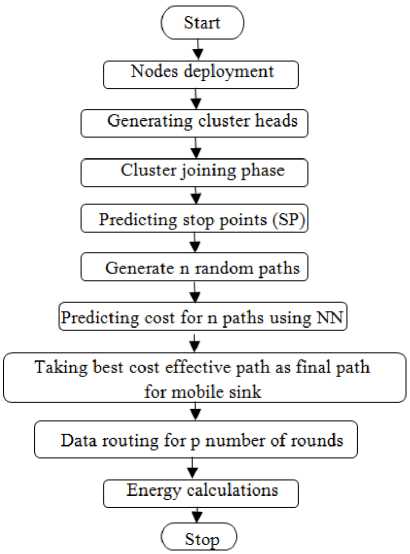
Fig.1. Experimental setup

Step 1: Nodes deployment: Nodes are deployed in a random manner in the given area.

Step 2: Generating cluster heads: cluster heads are generated considering energy, node density, number of hops.

Step 3: Nodes joining cluster heads: distance between the nodes and nearest cluster heads is calculated. Hence, least distance is used by node to join respective cluster head.

Step 4: Prediction of stop points (SP): Stop points are predicted by using distances between cluster heads. Cluster heads are selected as stop points as well as the distance between the cluster heads is calculated and compared with the twice of transmission range. If it lies between the range then the mid points are selected as stop points too.

Step 5: Generation of paths: n random pat are generated by trained neural network.

Step 6: Predicting the cost of paths: The cost of paths generated is estimated by the tour length.

Step 7: Final path selection: After the testing and training of the network, best path with the least tour length is selected by the trained neural network

Step 8: Data routing: as soon as the path is selected mobile sink visits the stop points for collection of data

Step 9: Energy calculations: the energies are calculated using standard formulae. Transmission and receiving energies are calculated.

• 4.    Proposed Work

In the proposed work mobile sink has to visit each of the stop point for collection of data. This process follows four stages, clusters head (CH) selection, CH joining phase, prediction of stop points, path selection using neural network (NN) and energy calculations.

• I.    Cluster head selection

Firstly all the nodes are deployed in random uniform manner. Fig. 2 shows the deployed sensor nodes with base station being in center. Node density, distance from the base station. Number of hops and residual energy are used to identify the cluster head. One hop distance is preferred in this work for the data transmission. According to the above listed features, ranking of all the nodes is done. One with the best of the features that is one at top rank is selected as first cluster head and so on. A check is made that next node to be selected as cluster head does not lie in the range of prior selected cluster head. To reduce to load on one cluster head, the reselection of cluster heads is done on the random basis after every ten rounds.

Following equations are to be followed for evaluating cost CH selection:

for i = 1 to i = n end

E ; = remaining energy of i th node

D_t = distance of i th node from sink

C_t = cost of i th node

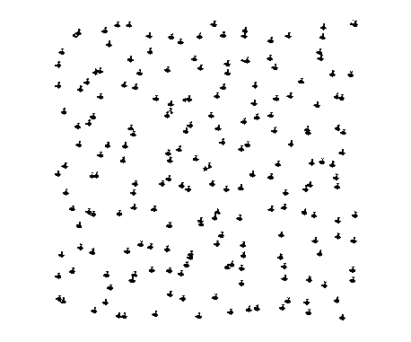
Fig.2. Sensor nodes

• II.    Cluster head joining phase

As the cluster heads are selected, members join them. Nodes falling in one hop distance join the nearest cluster head. If the node lies to two or more cluster heads within single hop distance, then the distance of the node is calculated with concerned cluster heads. The CH having minimum distance with the node is chosen as parent node.

for i = n to i = N min_dis = inf CH = 0

for j = 1 to C

d = J((CHXj - CHXi)2 + (CHyj - CH^) )1) x 0.5

if (d i j < min_dis)

CH = j endif end end

CH_X, CH_y = x and y positions ofj th cluster head

Nxi, Nyi = ith node location

C = number of elected cluster heads

• III.    Stop point selection

Once the cluster heads are selected, next step is the selection of stop points. Cluster heads are pre-selected as stop points.

Keeping cluster heads aside, few other nodes are also selected as cluster heads. For selecting those points distance between two neighboring CH’s is calculated. If this distance lies within range 2Tx_range, then midpoint of the distance is picked up as stop point. Criteria followed for it, is as follows for i = 1 to i = c-1

SPxi = (CHxi + СНХ(+)) x 0.5

end

Once all the stop points are selected then all of them need not be visited by sink. Unique stop points are selected.

• IV.    Selection of path using NN

After all the process being carried out, then comes the path selection. For selection of the best route, a neural network is trained. This machine learning based tool itself selects the path. Firstly the neural network is trained and secondly it is tested. Extracting features used to train neural network are distance from sink and cluster head selected. These features are used to generate output tour length. This trained network is then saved for further use. After training of the network, testing is to be done. This allows data communication. NN gives the reduced tour length due to which network life time is increased. Energy consumption is also less, so the hotspot problem is resolved. Load balancing is also done which improves the performance of network.

( Start )

Nodes deployment ;

Nodes clustering

CH’s election phase , T , Generate n number of routes

| Extracting features |

, г ,

| Training of NN using extracted features |

Store trained NN

C Stop )

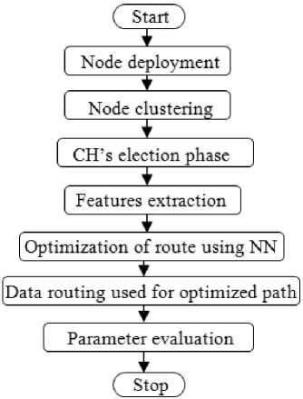
• Fig.3.    Proposed algorithm of neural network training

  

• Fig.4.    Proposed algorithm of neural network testing

Steps followed for training and testing of the artificial neural network are illustrated in fig. 3 and fig. 4 respectively. For the training phase after the selection of cluster heads and formation of clusters, extracting features such as cluster, distance between two cluster heads and sink distance are used to train the network. After training of the network, that network is saved. This saved network is used to obtain the desired results. While in the testing phase, after the training of network, paths are optimized and best one is selected. After the selection of the best path, data routing takes place that is sink follows the selected route for data collection. After the data collection evaluation of parameters is done depending on the need.

• V.    Energy calculations

For the energy calculations, transmission energies and the receiving energies are considered. When one round gets completed then the energy consumed in that round is calculate. For the node behaving as cluster head total energy consumed is sum of receiving energy and transmission energy. Receiving energy is the energy consumed while collecting data from other nodes. While, the energy of other nodes is just the transmitting energy.

Energy equation used for this purpose is the standard energy equations, as mentioned below:

E_TX(k, d) = kx E_elec + kx (E_amp x d²)                                                        (5)

E_RX(k) = E elec x k                                                                                (6)

Where,

E tx = transmitting energy

E rx = receiving energy

E _ei_ec = power per bit induced while transmitting or receiving

Eamp = amplifier coefficient for sending 1 bit d = distance between two nodes к = packet size.

• 5.    Simulation and Analysis

For the verification of the performance of the network, following performance metrics are studied:

• (1)    Network Lifetime: until the first sensor node dies out, number of rounds is calculated. These rounds show the life of network

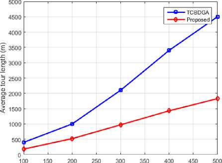
• (2)    Average Tour Length: length of the whole path followed by the mobile sink for collecting data.

The comparison carried out of the proposed work is with TCBDGA (Tree cluster based data gathering algorithm), keeping the simulation parameters same. Work carried is similar to that of TCBDGA but the difference lies in the path followed. The path followed in this work is optimized using a trained neural network .

Table 1. Simulation parameters

Parameter	Definition	Default value
E_int	Initial energy of each sensor node	0.5J
E_elec	Power per bit induced by transmitting or receiving network	50*10-9 J/bit
E_amp	Amplifier coefficient to send 1 bit	10*10-12J/bit/m2
N	Sensor nodes	100,200,300,400,500
Tx_range	Transmitting range of sensor node	10m,20m,30m,40m,50m
L	Side length of area	100m,200m,300m400m,500m
k	Packet size of data	2000 bit

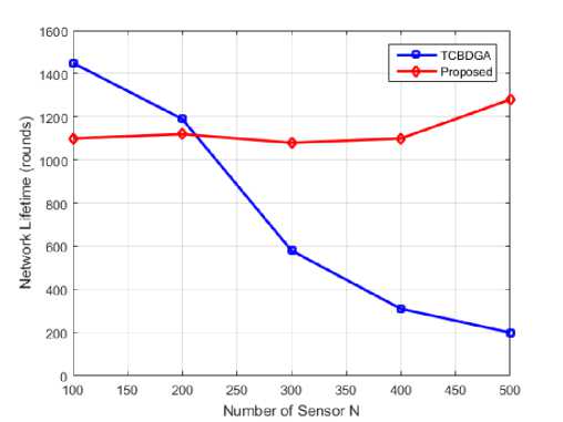
Fig.5. Network lifetime comparison

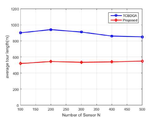
Fig.6. Average tour length of sink comparison on changing nodes reducing the tour length. TCBDGA has large tour length when the Tx_range is about 10m, as the range goes on increasing, tour length keeps on decreasing.

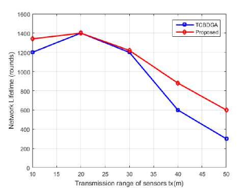
Fig.7. Average tour length of sink comparison on varying transmission range

When the transmission range of nodes is 20 m and 30 m, results produced by both algorithms are similar, the lifetime of the network, in that case, is quite same. As we keep on increasing the range of nodes, lifetime of network decreases but far better than TCBDGA. Further adding to it, as the range of nodes is increased, number of rounds fall down to a greater level. Both of these approaches are well suited for the lesser transmission range. For transmitting data at greater ranges leads to greater consumption of energy hence decreasing lifetime.

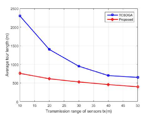
Fig.8. Average tour length of sink comparison on varying transmission range

Variation in tour length with range is depicted in fig 8. As the range is increased, a larger number of nodes are linked to each other. This reduces the stop points that are to be visited by the sink. This eventually results in a decrease of tour length.

• Effect of Changing Side Length of Area (L)

To study the impact of changing side length of the specified area, a number of sensor nodes are fixed to 200 and the transmission range is set to 30m. Fig. 9 shows the fluctuations in results of both the algorithms with an increase in area. A number of rounds are nearly similar to the area covered is 300m*300m. But as the area increases after 400m * 400m, lifetime tends to decrease but still far better than TCBDGA.

With the increase in area, average tour length of TCBDGA shows a sharp increase, as shown in fig. 10. Even though the area is increased but the tour length of the proposed algorithm is less than that of TCBDGA. When the area under observation is increased, nodes get distributed in that area .

To study the impact of changing side length of the specified area, number of sensor nodes is fixed to 200 and the transmission range is set to 30m.

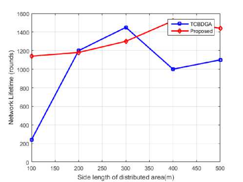
Fig.9. Average tour length of sink comparison on varying side length

Side length of distributed area(m)

Fig.10. Average tour length of sink comparison on varying side length

Nodes are much widely spread which leads to increase in tour length of the sink. The proposed algorithm always performed better than TCBDGA whether we talk in terms of number of rounds or its average tour length of the sink. Both the algorithms focus on load balancing and lesser energy consumption Keeping in account all the aspects, roposed algorithm produced bettere results. On varying side length of the area, network lifetime of both the approaches keeps on fluctuating. It can be clearly seen no proper pattern is being followed

• 6.    Conclusions

Path optimization by a trained neural network is studied in the paper. Results are compared to the results of TCBDGA. According to the observations made, the proposed algorithm is machine based learning that not only increased lifetime of the network but also reduced the tour length of the mobile sink. Further it adds to load balancing and reducing the energy consumption. It can be said that this approach is suitable for large areas as well as small areas for the collection of heterogeneous data.