Model Reference PID Control of an Electro-hydraulic Drive

Автор: Ayman A. Aly

Журнал: International Journal of Intelligent Systems and Applications(IJISA) @ijisa

Статья в выпуске: 11 vol.4, 2012 года.

Бесплатный доступ

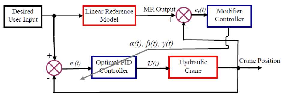
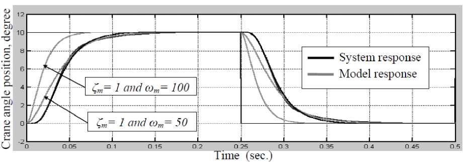
Hydraulic cranes are inherently nonlinear and contain components exhibiting strong friction, saturation, variable inertia mechanical loads, etc. The characteristics of these non-linear components are usually not known exactly as structure or parameters. For these reasons, tuning of the traditional PID controller parameters to control this system for the required performance faces a strong challenge. In this paper a new approach to design an adaptive PID control has the ability to solve the control problem of highly nonlinear systems such as the hydraulic crane was proposed. The core of the design method depends on comparing the performance of the Model Reference (MR) response with the nonlinear model response and feeding an adaptation signal to the PID control system to eliminate the error in between. It is found that the proposed MR-PID control policy provided the most consistent performance in terms of rise time and settling time regardless of the nonlinearities.

Еще

Hydraulic Crane, Nonlinear PID, Model Reference, Adaptive Control

Короткий адрес: https://sciup.org/15010328

IDR: 15010328

Текст научной статьи Model Reference PID Control of an Electro-hydraulic Drive

Published Online October 2012 in MECS

Electrohydraulic drives are widely used in industrial applications, such as in rolling and paper mills, as ‘‘actuators’’ in aircraft, and in many different automation and mechanization systems. The main reason for their broad industrial applications is the great power capacity that they can exert (as compared to their DC or AC counterparts), while preserving good dynamic response and system resolution, [1].

Hydraulic systems consist of various elements: pumps, actuators, control valves, accumulators, restrictors, pipelines and the like, which include many types of nonlinearities, such as pressure-flow characteristics in control valves, dry friction acting on actuators and moving parts of valves, collision of valves against valve seats, [2]. It is a marked feature of nonlinear systems that global behaviors are sometimes quite different from local behaviors. In such cases, results of linear analysis are unavailable to estimate global nature of the system.

Systems containing fluid power components offer interesting and challenging applications of modern and classical control techniques. The use of microcomputers and many feedback devices for hydraulic drives allows for implementation of different control algorithms that result in better steady-state and dynamic performances in fluid power control systems. There are a number of research results on the applications of adaptive control [2], robust control [3], and variable structure control [4] in electrohydraulic control systems.

In the Sliding Mode Control (SMC) method, the system trajectory is forced to reach the sliding surface and to slide along it, or to remain in its vicinity, [4]. Since in many situations the SMC is found robust to a great extent to plant parameter variations or uncertainties in the model of the system to be controlled, it has found broad applications. However, the chattering is a signify problem in the SMC implementations and solutions that either reduce or eliminate it had been investigated in [5, 6].

In a parallel way, even though fuzzy logic controllers often produce results superior to those of traditional controllers [7], the control engineer has found difficulties in accessing the fuzzy logic controllers because of the following limitations: The design of the fuzzy logic controller is not straight forward due to heuristics involved with control rules and member-ship functions. There is no standard systematic method for tuning the fuzzy logic controller parameters.

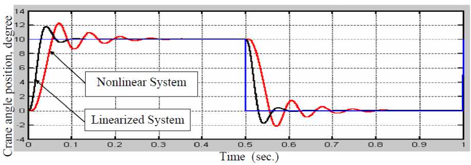
Gholamreza and Donath [8] recognized that a hydraulically actuated system contains a host of nonlinear elements, thereby making a linear controller ineffective. Furthermore, the authors illustrated that linearization of the dynamic equations over a small operating range and the design of an appropriate controller for each condition had limitations in the face of time variable parameters changes.

Most of the recent work performed on hydraulically actuated linkages has focused on developing some type of adaptive controller, [2, 3]. These controllers are meant to compensate in real-time for nonlinear elements such as friction and smooth time-variant load changes. These methods rely on continuous noise-free feedback and are generally computationally intense making them non-ideal for application to low cost mobile equipment.

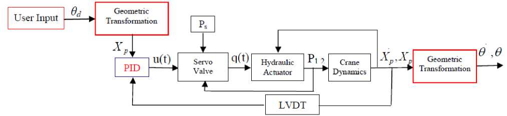
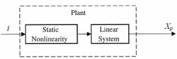
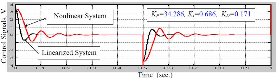
The aim of this paper is to design a nonlinear PID control has the ability to solve the control problem of highly nonlinear systems such as the hydraulic crane, which is shown in Fig.1. This will be done by first deriving a nonlinear mathematical model of the system and then approximating the transfer functions in the model by low order linear transfer functions. Using the low order linear transfer functions, design optimal gains of the PID regulator is determined. The final step is implementing the designed PID controller in the nonlinear model and then comparing the performance of MR response with the nonlinear model and feeding a correction signal to tune the PID control system parameters to eliminate the error in between.

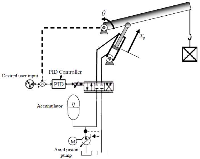
Fig. 1: Hydraulic Crane System

II System Construction

The servo system is composed of a hydraulic power supply, an electrohydraulic servo valve, a cylinder, mechanical linkages, and control. The piston position of the cylinder is controlled as follows: Once the voltage input corresponding to the desired position is transmitted to the servo controller, the controller signal current is generated. Then, the valve spool position is changed according to the input current applied to the torque motor of the servo valve. Depending on the spool position and the load conditions of the piston, the rate as well as the direction of the oils supplied to each cylinder chamber is determined. The motion of the piston then is controlled by these oils.

If it is necessary to represent servo valve dynamics through a wider frequency range, a second-order transfer function must be used. The relation between the servo valve spool position x v and the input current i v can be written as, [2]

d 2 xv dt 2

dx     2

+ 2^v^v —77 + ^v xv dt

= ®v k v i v

where kv represents the gain of the servo valve, ωv is the natural frequency of the servo valve, and ζ v is the damping ratio of the servo valve.

Fig. 2: Characteristic of the dead zone

The valve spool occludes the orifice with some overlap so that for a range of spool positions there is no fluid flow. This overlap prevents leakage losses that increase with wear and tear. Thus, the dead zone should be placed between the valve dynamics and actuator/load dynamics. For the sake of simplicity, this dead zone is equivalently moved to the position between the output of the controller and the input current of the valve. So, the dead zone nonlinearity may be characterized as shown in Fig. 2 and approximately described as:

iv

i -11   ifi > 11

<0          iflil < 11

i + Ix   if i < - I,

where i v is the current from the controller and I 1 the width of the dead zone.

The equations of the servo valve flow to and from the actuator (assuming symmetric valve port, zero lap design and zero return pressure) are as follows,

For positive x v

q, = CdWX, sgn( Ps - Pf )I2 P - Pf\

, qn = CdWxv sgn( Pn KpPI ' p                     (3)

For negative xv

q, = CdWxv sgn(P,)J|P|

,

qn = CdWxv sgn(Ps - P )l2 Ps - Pn|

V p                 (4)

where x v is the spool displacement, P s is the supply pressure, p is the mass density of the oil, Cd is the discharge coefficient of the orifice, W is the width of the orifice, suffix n denotes the annular side and suffix f denotes the full side.

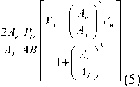
The linearized flow equation of the actuator is given by [8]:

The motion equation of the crane is given by

PleAe = MeXP + Bg Xp + Fd

where M e represents the equivalent mass of both the variable inertia load and the piston, B e is the equivalent viscous damping coefficient, and Fd represents the disturbing forces like friction forces.

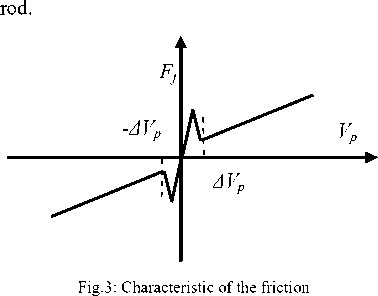
The various friction characteristics depend on lubrication, relative velocities of bodies at the contact point, pressures and others [1, 2]. A typical friction characteristic is presented in Fig.3. The mathematical description of friction process in hydraulic cylinders involves serious difficulties caused by:

  •    Presence of a wide range of different sealing elements in dynamic connections (O-rings, V-type seals, packing seal).

  •    Applications of various sealing materials rubbers or composite materials.

  •    Influence of temperature on friction resistance due to the fact that sealing materials have higher thermal expansion coefficient than metal elements.

Deposition of solid contaminations on the piston

Ae q = KA

1 +f A T

I A , J

1 +f A *-

I A f J

.

P ie + A e X P +

Thus exact simulation of the nonlinear behavior of friction in the vicinity of a zero velocity is difficult. The friction force is approximately simulated by the stick-slip friction law. The value of the stick-slip friction for positive values of Xp is given simply by where

Ple

p$A$ - P n A n    n _q , + q n , _A , + A n

A     ’ q e =    2    , Ae =     2

ГFst   for 0 < VP

=

f  [Fsi   forVp >A Vp

,

Ple is the effective load pressure, qle is the effective load flow rate, Ae is the effective piston area, B is the oil bulk modulus, k1 is the leakage coefficient of the piston, Xp is the piston displacement, Vn is the oil volume under compression in the annular side of the cylinder, Vf is the oil volume under compression in the full side of the cylinder, An is the annular area of the cylinder, Af is the full area of the cylinder.

where Fsl is the slip friction, Fst is the stick friction, and Vp is the piston speed .

The dynamics of hoses and pipes connecting the servovalve and the actuator are simulated by a time delay function. The transport lag function is given by

H ( s ) = e- sTd

Transport delays are approximated by a first-order lag

e

sTd

5 + 1

where Td is the delay time. The approximation introduces an extra pole to the system transfer function,

but, unlike Pade's method, it does not introduce an extra zero, [2].

The actuator is equipped with one hydraulic accumulator in the supply port to cope with the dynamic flow demands. A LVDT position transducer measures piston displacement with gain of 0.1 m/V. The block diagram of the hydraulic crane system is shown in Fig. 4. The system geometric transformation and its physical parameters are illustrated in Appendixes-A and B.

Fig. 4: Block diagram of the hydraulic crane system

III Controller Design

PID-controller is the most common in many industrial applications and it has been stated in many papers that a PID-controller has been used in hydraulic position servo systems [2, 3, 9, 10 and 11]. It is very natural solution to the controller of a type 0 system (velocity control, temperature control, pressure control). A position servo system is, however, a type 1 system, and this means that there is already an integrator in the forward loop (actuator, cylinder, or motor). On the basis of the understanding obtained from the analysis of plant dynamics and its nonlinearities, one can a set of control requirements. The most serious nonlinearities are the nonlinearities of valves, load, and friction forces. According to linear theory of hydraulic servo systems the nonlinearities, which are in the forward loop before the integrator as shown in Figure 5, cause the position error in position servo systems, and it is responsible for performance limitations. Unquestionably, the plant as a whole poses a very difficult dynamics to control.

Fig. 5: Model of the hydraulic drive system

As detailed model of the crane would be difficult to derive so it is too complex to be used in regulator design. The common solution is often at first approximate the real complex model to linearized one and finally adjust nearly the PID controller parameters according to standard design method such as Ziegler-Nichols, [12] method which is considered in the most popular one during the last 50 years. The linear PID-control algorithm in Laplace form is presented as follow,

U ( 5 ) =

Kp +--I- + KdS

s

E ( 5 )

where U(s), E(s) are the controller output and system response error, KP, KI, and KD are the proportional, integral and derivative PID gains respectively. According to the studies of many researchers in the field of fluid power control systems, [3, 4, 5 and 7] the following conclusions can be made:

Linear PID-controllers are not suitable controllers for hydraulic position servo because of overshoots and limit cycles. Since PID controller parameters are usually designed using either one or two measurement points of the system frequency response as Ziegler-Nichols method, their control performance may not satisfy the desired time-response requirements.

Fig. 6: Block Diagram of Crane hydraulic Control System

When a system has different operating points with widely differing dynamic properties and high position accuracy is required, it is not always possible to control it with a fixed parameter controller, a nonlinear design of PID-controller might be a solution. So it seems a good idea to use a model reference control system based on PID control policy can guide the system regardless the exit nonlinearities. The proposed scheme is shown in Fig. 6.

The steps of the proposed control strategy is as follows,

The first step is approximating the nonlinear hydraulic crane model to linearized one by ignore all nonlinearities and design an optimal PID controller for it. In order to have a good closedloop time response, the following performance function needs to be considered during the design of the PID controller parameters:

Gm(s) =

ωm2

s 2 + 2ζ ω s + ω2

mm   m

where the parameters ωm is the model natural frequency and ζm the model damping ratio, which are chosen according to the desired time-domain response requirements of the closed-loop system.

The forth step is modifying the nonlinear model response by comparing it with the MR response and fed a modifier signal to eliminate the error in between of them by correction the PID controller action.

Using modifying law similar to Equation (10), one obtains the rules base for the modifier controller. The variations in the PID gains will be as follows:

J(K ,K ,K ) =ITASE

where ITASE is the integral time absolute square error of the system output. Thus, the optimal PID controller design problem may be stated as

J

KP ,KI ,KD

(KP,KI,KD)

The second step is implementing the optimal designed PID controller in the nonlinear model. Of course the system response will be worth than the response of the linearized one.

K = α(t) K

,

KI = β(t) KI ,

KD =γ(t) KD ,

α(t) = Kpmer (t),

β(t) = KIm∫ er (t)dt and de (t)

γ(t) = KDm   r dt

The third step is defining the reference model, in the time domain; specifications for a control system design involve certain requirements associated with the time response of the system. The requirements are often expressed in terms of the standard quantities on the rise time, settling time, overshoot, and steady-state error of a step response. The time response of a standard second-order system is widely used to represent the above timedomain requirements as a model reference to the real nonlinear time variant system. Thus, the second-order system is chosen for the tracking mode, whose transfer function is

where er(t) is the relative error between the MR and the system response, cer(t) is change in the relative error, ∆KP, ∆KD, and ∆KI are the PID gains variation, KP, KD, and KI are the calculated gains of the PID controller based on Equation (12), α(t), β(t) and γ(t) are the modifier outputs and  KPm, KIm and KDm are scaling factors.

IV Simulation

The continuous PID was automatically converted to a discrete form with sampling period was chosen to be 0.001 sec. by considering the fast plant dynamics. The cost function was given by J(KP, Kl , KD). The reference

input was a step signal, which changed from 0 to 10 degree. Using the MATLAB optimization toolbox, the optimal PID parameters KP=34.286, Kl= 0.686 and KD=0.171 were found (to three decimal places, thereafter).

Figure 7.a shows the closed-loop responses due to step input of linearized and nonlinear model with the optimal PID controller which, was designed based on the linearized model. It is clear that the difference in the two responses due to the nonlinearities of the system which appears as increasing in the overshoots, rise time and settling time however, the steady state error is zero in the two cases. The corresponding controller signals for each case are shown in Fig.7.b.

Fig. 7-a: Step response of closed loop systems with different settings

Fig. 7-b: The control signals based on optimal PID Controller

Fig. 8-a: Step response of the system based on the proposed controller

Since in many industrial applications, it is necessary to assure that the response has minimum/no overshoot, this is achieved in Fig.8.a which, illustrates the model reference responses and the nonlinear system responses based on the proposed control policy with model damping ratio (ζm= 1) and two suggested model natural frequencies (ωm= 50 and 100 rad/sec). It easy to decide the value of ζm to be critically damped however the value of ωm need extra effort to be chosen within the physical limitation of the cylinder maximum velocity. It is noticed that the responses are improved compared with the responses of Fig.7.a where, there is smaller settling and rise times with no steady state error or overshoot. In the nonlinear PID controller design, a higher level is the model reference controller, which, at any instant, evaluates control performance and adapts the output of the controller according to the relative error in the performance of the reference model and the nonlinear system responses.

The parameters of the modifier controller were KPm=1.45, KIm=0.720 and KDm=0.140. The crossholdings controller outputs of the proposed strategy for the tested model are illustrated in Fig.8.b. It is interesting to notice that the amplitude of controller’s signals became smaller with implementing the proposed strategy compared with Fig. 7.b, which is signifying index in the hydraulic system design and in its power energy saving.

Figure 8.c represents the modification signals in the PID control of the nonlinear system with the two tested models. It is a remarkable notice that the modification mechanism work only with the transient change in the system response.

Another good application with sinusoidal input signal as a continuous motion test for the proposed controller policy with the nonlinear system is shown in Fig.9. The system response follows the model reference with delay of 17 msec.

Fig. 8-b: Controller signals

Fig. 8-c: Modifier controller signals

10 - ■ ■

5 -

System responseReference Input

-5 - ■

1 and com= 100

Model response

-to -

О 0.2     0.4     0.6     0.8

1.2     1.4     1.6     1.8

Time (sec.)

Fig. 9: Sin wave response of the system based on the proposed controller

V Conclusions

Nonlinear dynamic phenomena in hydraulic systems are unique and diverse. It is difficult to estimate their global nature from local nature by linear analysis. Thus, the hydraulic systems are often very conservatively tuned. In addition the fact that the cost of getting the tuning wrong can be highly destructive and costly. To effectively assess the performance of the proposed tuning method, the control system performance is evaluated via simulations.

In this paper the position control problem of a hydraulic crane was addressed. The highly nonlinear behavior of the system limits the performance of classical linear controllers used for this purpose. It has been demonstrated that the MR-PID control can be successfully implemented in the control system of a hydraulic crane. Since there are nonlinearities in the hydraulic position control system, it is difficult to achieve high-precision tracking performance using only linear PID controllers. The results obtained show that the proposed controller policy exhibits much better response, much better tracking characteristics, and retains excellent following motion property comparable to, or better, than that obtained by the conventional optimally tuned PID controller.

In addition to faster and more accurate responses, the proposed controller design steps are simple, thus, the application of the algorithm can be made wider than that of the conventional PID controllers.

Список литературы Model Reference PID Control of an Electro-hydraulic Drive

  • H.E. Merrit, “Hydraulic control systems”, John Wiley & Sons, 1976.
  • J. Watton. “Fluid power systems: Modeling, simulation, analog and microcomputer control”, Prentice-Hall International, London, UK, 1989
  • J.W. Dobchuk, “Control of a Hydraulically Actuated Mechanism Using a Proportional Valve and a Linearizing Feedforward Controller”, PhD, Department of Mechanical Engineering, University of Saskatchewan, Saskatoon, Canada, Aug. 2004.
  • A. Bonchis!, P. I. Corke, D. C. Rye and Q. P. Ha, “Variable Structure Methods In Hydraulic Servo Systems Control”, Automatica (37), pp 589-595, 2001.
  • Daohang Sha a, Vladimir B. Bajic b and Huayong Yang, “New Model and Sliding Mode Control of hydraulic Elevator Velocity Tracking System”, Simulation Practice and Theory Journal (9), pp 365–385, 2002.
  • G. Bartolini, A. Ferrara and E. Usai, “Chattering Avoidance By Second-Order Sliding Mode Control”, IEEE Trans. Autom. Control 43 (2), pp 241–246, 1998.
  • Ayman A. Aly and A. Abo-Ismail, “Intelligent Control of A Level Process By Employing Variable Strcure Theory”, Proceeding of International Conference in The Mechanical Production Engineering, Warso, Poland, 1998.
  • Ayman A. Aly, Aly S. Abo El-Lail, Kamel A. Shoush and Farhan A. Salem “Intelligent PI Fuzzy Control of An Electro-Hydraulic Manipulator” I.J. Intelligent Systems and Applications, 7, 43-49, 2012.
  • Sepehri, N., Lawrence, P.D., Sassani, F., and Frenette, R., “Resolved-Mode Teleportation Control of Heavy-Duty Hydraulic Machines”, ASME Journal of Dynamics Systems, Measurement and Control, V116, N2, pp 232-240, 1994.
  • Ayman A. Aly, and H. Ohuchi “Fuzzy Hybrid Control Using Indirect Inference Control For Positioning An Electro-Hydraulic Cylinder”, Conference of Fluid Power System, Yamaguchi, JAPAN, 2001.
  • Wilson J. Rugh, “Analytical Framework for Gain scheduling”, American Control Conference, San Diego, California, USA, May 1990.
  • Ziegler, J. G., & Nichols, N. B., “Optimum Settings for Automatic Controllers”, Transactions of ASME, 64, pp 759-768, 1942.
Еще
Статья научная