Modeling Changing Graphical Structure

The estimation of large-scale covariance matrices from data is a common problem, with applications in many fields, ranging from bioinformatics to finance. For multivariate Gaussian data, this problem is equivalent to model selection among undirected Gaussian graphical models. The graphical models have been shown to be valuable for evaluating patterns of association among variables[1]. For an introduction to graphical models, we refer to [2-4]. A mathematical rigorous treatment can be found in [5].

Dempster (1972)[1] has introduced graphical approach to modelling the variance-covariance matrix in which zeros in the inverse covariance matrix(the precision matrix) correspond to conditional independence properties among the variables, as well as to missing edges in the associated graphical model. In this setting, a sparse inverse covariance matrix, if it fits the data well, is very useful to practitioners, as it simplifies the understanding of the data.

Sparsity is also often justified from a statistical viewpoint, as it results in a more parsimonious, and also more robust model. So the graphical models have become an important tool for analyzing multivariate data

• * Corresponding author.

• 2.    Our Approach

and have been successfully applied to genetics[6], medicine[7] and economy[8].

In the case of univariate time series, segmentation might be induced by a change of mean or variance. But in the case of multidimensional time series, we can additionally segment if the correlation structure changes. Such changes are often much harder to detect, but often arise in practice, especially in areas such as finance. Recent research shows that correlation differs between volatile and tranquil periods[9-10].The time-varying variance-covariance matrix has been widely accepted.

Talih (2003) [11] focuses instead on the latent graphical structure related to the precision matrix. They developed a graphical model for sequences of Gaussian random vectors when changes in the underlying graph occur at random times, and a new block of data is created with the addition or deletion of an edge. They applied their methodology to study multivariate financial data. However, they assume that the graph structure changes slowly over time, which violates the assumption that the parameters of each model in each segment are independent.

In this paper, the model of Talih is developed and we assume the graphical structure of each block is independent. Given parametrization, the algorithm is designed by MCMC method. At last, the time-varying dependency structure is applied to the stock market in China.

Consider the sequence of graphs which arises in blocks as follows:

G1,   ,G1,G2,   ,G2,   ,GB,   ,GB                                                               (1)

N1N2                NB where the graph G in block b is repeated a random number of times N : Each graph G is an undirected graph with fixed vertex set V= {1,   ,d} and edge set E .

For each graph G , variance-covariance matrix ∑ of d-dimensional multivariate Normal random vector, constrainted in such a way that its inverse, the precision matrix K ,belongs to the set M ⁺ ( G ) . For any undirected graph G ( V , E ) , the set M ⁺ ( G ) is defined as the set of all symmetric and positive definite matrices K . Thus, for graphical Gaussian models, ( i , j ) ∉ E if and only if k 0.

For a given block b with precision matrix K ∈ M ⁺ ( G ) and undirected graph G ( V , E ) , we follow Talih (2003) and Zhang(2007)[12] and parameterize the precision matrix K ( k ) _х as follows:

b    vi      b        θb kii =    2   ，kij =-            ×I{(i,j)∈E ,i≠j}

• ^σ i , b              ^σ i , b ^σ j , b            ^b

where I denotes a indicator function, ( i , j ) represents the edge between vertices i and j , v_i^b = max(1,#{ j :( i , j ) ∈ E_b }).

In order to keep K positive definite, we have to limit |6     1 .

We view the data as a stream of d-dimensional observations

Y ,    ,Y ,Y • • • К • • • У . • • • У

• 1,1 ,     , 1, N ₁ , 2,1 ,     , 2, N ₂ ,     , B ,1 ,      , B , N_B

N1N2                   NB where the block lengths N,,N are random conditional on the number of blocks B , and a fixed sample size n ,the last block has length

B - 1

NB=n-∑Nb b=1

Let G = ( G ,   , G ) and N = ( N ,   , N ) , the full data can be represented as follows:

( Y , G , N ) = {( Y 1 , G 1 , N 1 ),  ,( Y B , G B , N B )}

Here, each Y is a d× N matrix with column vectors Y ,   , Y . Data in block b are assumed independent and identically distributed from N (0, ∑ ) ,with the precision matrix K = ∑b-1 ∈ M+(Gb).

The log-likelihood function for Y given the sequences G , N and K is log f ( Y | K , G , N )

=- ^nd log(2 π ) + ∑ ^BNb log K b - ¹ ∑ ^Btrace ( K b Y b ′ Y b ) 2                b = 1 2               2 b = 1

T he joint posterior distribution of parameters is given f ( G , θ , σ , N | Y ) ∝ f ( Y | G , θ , σ , N ) ⋅ p ( G ) ⋅ p ( N ) ⋅ p ( θ ) ⋅ p ( σ )

• 3.    Algorithm

It is difficult to get the solution from (2) directly, we consider to draw the sample from the joint posterior using monte carlo simulation. For this purpose, we apply Gibbs and Metropolis-Hastings(M-H) iterative method. Given the conditional posterior distributions, we implement the sampling to generate sample draws. The following steps can be replicated until convergence is achieved.

Step 1: We use the simple case, θ ≡ θ and σ ² ≡ σ ² for all b . Specify starting values for the parameters: θ , σ , G , B and N .

For the prior distribution of and σ ² ,we follow Talih(2003) and Zhang(2007) to assume that

p(θ) ∝     π/2     , p(σi2)∝1 (i=1,, cos2(θ⋅π/2)

For undirected graph G , there are at most d ( d - 1)/2 edges. We assume that each graph has the same prior probability, i.e. the prior distribution of G of each block is described as follows:

p(Gb)=2-d(d-1)/2  (b=1,,

In the thesis, we assume that B is fixed and N ( b = 1,   , B ) follows a uniform(Maxwell-Boltzmann)

distribution over the space of vectors.

Step 2: Generates G ^new , σ ^new and θ ^new from p ( G | Y , N ) , p ( σ | Y , N ) and p ( θ | Y , N ) using M-H algorithm.

® M-H design for graph G

We consider M-H design of G_b by changing graph from G old to G_b new and keep в , Q , G__b and N unchanged, where G represents the remain graph except G .We assume that at most one edge is changed from G^old to G^new .With the assumption of equal probability, the designed conditional probability density q ( G^new | G^old ) is as follows:

q(Gn™ | G°ld ) = 2—d(d-1)/2 (b = 1,•• •, B)

Similarly,

q(G°ld | Gnew) = 2—d(d-1)/2  (b = 1, • • •,B)

The acceptance ratio of iterative for graph G is given by old    new

a(Gb , Gb  )

f ( Y , G b^new

= min <  1,

,G-ьв,Q,N) x q(G7 | G°ld)\

f (Y, G°ld, G—b, в, Q, N)   q(G°ld | G7 ) 1

= min 1 1,

f (Y | G"”, G—b ,в, q, N)

[ , f (Y | G°ld,G—b,в,Q,N)

@ M-H design for в

Keeping G , Q , N unchanged, we consider M-H design of в . We assume that tan( 0n / 2) follows the random walk:

tan(Onewn / 2) = tan(e°ldn /2) + £where £ ~ N(0,0.81).

Simple computation shows that the acceptance ratio for parameter в is given by

ав,в-) = min 11, fWG^,Q,N) i I  f (Y|G, ff", q, N) J

® M-H design for Q

Keeping G , в , N and Q__z unchanged, where Q__z represents the vector left by removing ^ from

Q ,we consider M-H design of Q .We assume that log( ^ ²) follows the random walk:

log(^- new ) = log("",2old ) + £ where £ ~ N(0,0.625).

Then the acceptance ratio for parameter ( 7 _z is given by

^{a (} ^ / 2 old ,^^, new ) = ^min I ^1,

f ( Y | G , в , q -„а 2 new, , N ) f ( Y | G , в , q - , ., a ; 2 °_и , N )

Step 3: Generate N ^new from p ( N | Y , G ) using Gibbs sampling algorithm.

Proposals on the vector of block lengths can be made locally in the sense that only two components of N = {N^, Nb } are changed at any given time. Indeed, draw some b G {1,-* •, B} is drawn at random. Then, a symmetric proposal N = {New, •. *, N^w } can be constrained only by new      new      old      old

Nb + Nb+1 = Nb + Nb+1

The acceptance rate for the shift move is given simply by a ( N od , Nⁿ™ )

= min <  1,

f ( Y b | G b , 9 , o ,N ) f ( Y b + 1 1 G b+ 1 , e , a , N^ ) f ( Y b | G b , 9 , o ,\ ) f ( Y b + 1 1 G b+ _v, 9 , a , N^ )

Step 4: go to step 2. Step 2 through Step 4 can be iterated S times to obtain the posterior densities. Note that the first L times iterations are discarded in order to attenuate the effect of the initial values.

• 4.    Simulation

We generate the sample ,which consists of 400 independent observations drawn from a multivariate Normal distribution with mean vector zero, and a precision matrix constrained by the graph in Fig. 1, and parameterized by

9 = 0.97, q = {0.3,0.25,0.3,0.25,0.3}

Then there are two blocks in our simulated data of length

N = ioo, N = 300

Q

Q

О

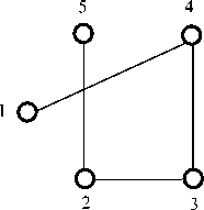
Fig. 1 The original graphical structure

We would like our proposed method to recover that fact. We use 10000 replications in MCMC algorithm and discard first 1000 draws of the chain. The posterior properties of parameters are given in table 1. The posterior median of 9 is slightly larger than the true value, while the median of Q is slightly smaller than the original value. From the posterior property of N , we detect the change point exactly. It is more important that both the posterior graph of each block are exactly the true graph.

Table 1 The posterior properties of parameters in simulation

	θ	σ 1	σ 2	σ 3	σ 4	σ 5	N 1
Median	0.9838	0.2460	0.2325	0.2530	0.2304	0.2610	100
Mean	0.9838	0.2461	0.2327	0.2532	0.2305	0.2612	100.2
Min	0.9796	0.2320	0.2202	0.2374	0.2171	0.2487	99
Max	0.9876	0.2635	0.2480	0.2708	0.2445	0.2824	103
Std	0.0011	0.0051	0.0044	0.0049	0.0043	0.0051	0.72

• 5.    Application

  In this thesis, we choose to work at the portfolio level using five industry index: Real states, Industries, Commerce, Public utilities and Integration in the Shanghai stock market of China. We select sample from October 1996 to December 2005, providing 111 months of data. The dataset is obtained from by data library of CSMARS in China. We follow Talih (2003) and assume monthly log returns is multivariate Normality, and center the observations around their sample mean in order to focus only on the precision matrix.

In application, we assume there is two blocks in the shanghai stock market. We discard first 1000 draws of the chain and use the remaining 9000 observation to find posterior distributions of the parameters.

Table 2 The posterior properties of parameters

	θ	σ 1	σ 2	σ 3	σ 4	σ 5	N 1
Median	0.9733	0.0376	0.0406	0.0451	0.0337	0.0413	47
Mean	0.9727	0.0377	0.0407	0.0452	0.0337	0.0414	46.7
Min	0.9547	0.0330	0.0348	0.0378	0.0286	0.0364	40
Max	0.9824	0.0436	0.0488	0.0555	0.0415	0.0488	65
Std	0.0044	0.0016	0.0018	0.0022	0.0016	0.0017	3.1

Commerce

Industries

Real states

Integration

Public utilities

Fig. 2 The graphical structure of stock market in China

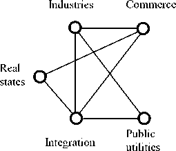
Fig. 2 shows that there is obvious different graphical structure between the different blocks. We name the first block as “weaker correlation”, as there is five edges in the first graphical structure. The second block is named as “stronger correlation”, as there is seven edges in the second structure.

Table 2 shows that the median of N is 47, which denotes that the change point happens on October 2000 or so. From October 1996 to September 2000, there is the weaker correlation. From October 2000 to December 2005, it enters the stronger dependency structure. In fact, from 1999 to 2001, there is the bull market in China, while from then, China enter into a span of four years of bear markets. The result is consistent with the view that a bear market reflects high correlation, while there is low correlation in a bull market.

• 6.    conclusion

The changing dependency structure based on graphical model is proposed in the paper. The markov chain monte carlo method is applied to design the algorithm. The numerical simulation demonstrates the algorithm is effective. The model and algorithm are applied to study the conditional dynamic relativities of five segments of the market in China. Empirical results show that the dependency structure is time-varying. In the first block, the correlation is comparatively weaker, while the second block is accompanied with stronger dependency structure. Our results indicate that a bear market is associated with the stronger dependency, while there is the weaker dependency in a bull market.

The method can be applied to the portfolio construction and value at risk measures if returns follows multivariate Normal distribution. Our empirical distinction between bear and bull markets has potential implications for the optimal allocation of assets.