Modeling, Simulation and Control Issues for a Robot ARM; Education and Research (III)

Published Online March 2014 in MECS

The accurate control of motion is a fundamental concern in Mechatronics applications, where placing an object in the exact desired location with the exact possible amount of force and torque at the correct exact time is essential for efficient system operation [1]. This paper extends writer's previous works [1,2], the ultimate goal of this work addresses design, Modeling, simulation and control issues for robotic arm, Particularly, to design a robot arm, select and apply different control strategies, so that an applied input voltage with a range of 0 - 12 volts corresponds linearly to an output arm angle of 0 to 180, The designed system should respond to the applied input with an overshoot less than 5%, a settling time less 2 second and a zero steady state error, as well as, to simplify and accelerate the process of robot and control design and analysis, two suggested MATLAB function block models with its function block parameters for robot arm design, control selection and analysis purposes to be proposed.

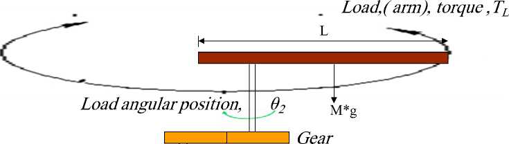
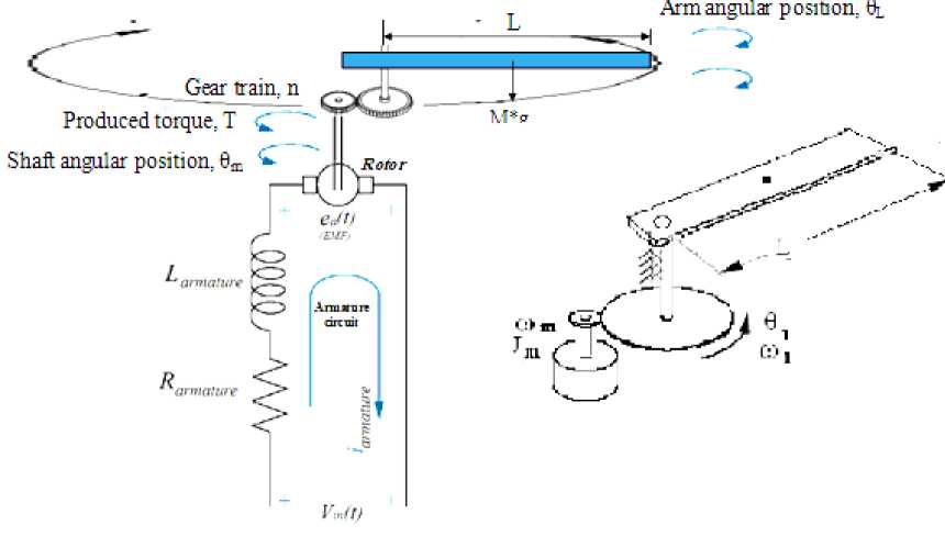
Having both electrical and mechanical parameters, a single joint robot arm is an application example of a Mechatronics electromechanical system used in industrial automation. Each degree of freedom (DOF) is a joint on Robot arm, where arm can rotate or translate, each DOF requires an actuator, A single joint Robot arm is a system with one DOF that is one actuator, when designing and building a robot arm it is required to have as few degrees of freedom allowed for given application. As shown in Figure1 , PMDC motor is, widely, used as an electric actuator to drive a robot arm horizontally. The motor system input signal used to provide the control voltage and current to the PMDC motor is a voltage signal. In part I [1] to simplify and accelerate the process of DC motors sizing, selection and dynamic analysis for different applications, using different approaches, different refined mathematical models in terms of output position, speed, current, acceleration and torque, as well as corresponding Simulink models, supporting MATLAB m.file and function block models are introduced for comparison and analysis purposes were introduced. In part II [2] addresses a comprehensive study and analysis of most used control strategies of a given DC motor for comparison and analysis purposes, to select the best and most suitable control strategy for specific motion application, e.g. to control the output angular position, θ and speed of a given DC motor, used in Mechatronics motion application. These works are intended for research purposes, as well as for the application in educational process. In [3] to simplify and accelerate Mechatronics motion control design process including; performance analysis and verification of a given electric DC system, proper controller selection and verification for desired output speed or angle, a new, simple and user–friendly MATLAB built-in function, mathematical and Simulink models are introduced

• II.    System Modeling, Simulation, Characteristics And Analysis

In modeling process, to simplify the analysis and design processes, linear approximations are used as long as the results yield a good approximation to reality [3]. As shown in Figure 1, Single joint robot arm system consists of three main parts; arm, connected to actuator through gear train with gear ratio, n [4]. Because of the ease with which they can be controlled, systems of DC machines have been frequently used in many applications requiring a wide range of motor speeds and a precise output motor control [5-6]. The robot arm system to be designed, has the following nominal values; arm mass, M= 8 Kg, arm length, L=0.4 m, and viscous damping constant, b = 0.09 N.sec/m. The following nominal values for the various parameters of eclectic motor used: Vin=12 Volts; Jm=0.02 kg·m²; bm =0.03;Kt =0.023 N-m/A; Kb =0.023

V-s/rad; R a =1 Ohm; L a =0.23 Henry; T Load , gear ratio, for simplicity ,n=1.

Motor angularposition, θ1

Motor torque ,Tm

Z

(a)

Y

X

(b)

Fig. 1(a)(b): Simplified schematic model of a single joint (one DOF) robot arm and DC motor used to drive arm horizontally

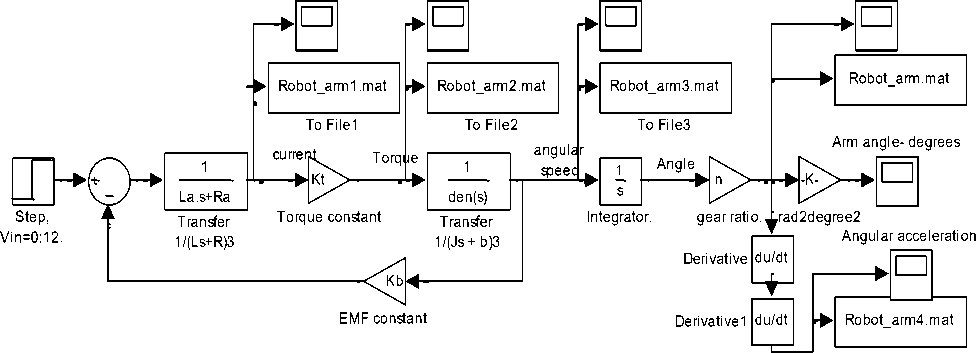
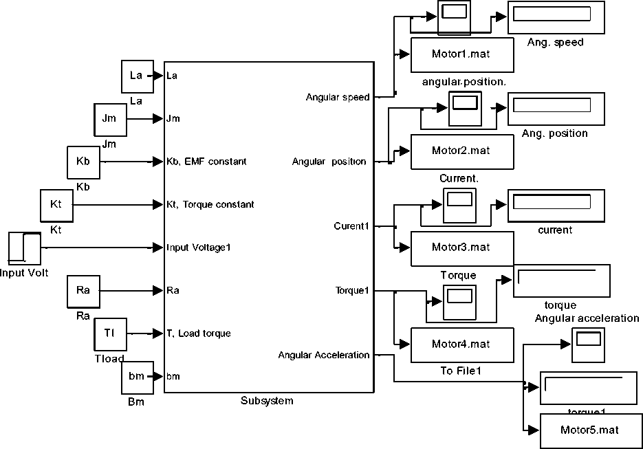
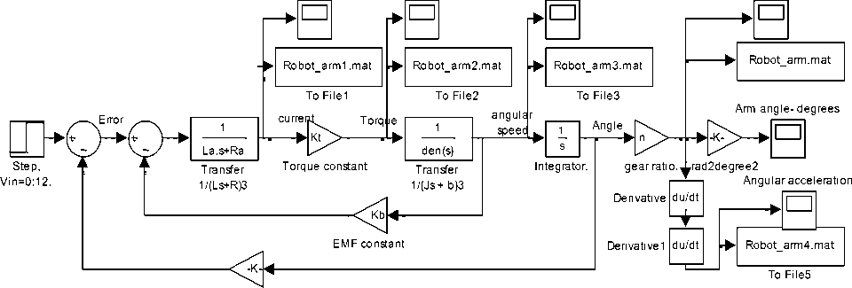
Based on the Newton’s law combined with the Kirchoff’s law, the mathematical model of PMDC motor in the form of differential equations or state space equations, describing electric and mechanical characteristics of the motor can be derived. In [2-4], based on different approaches, detailed derivation of different refined mathematical models of PMDC motor (e.g. Eqs (1-2)) and corresponding Simulink models are introduced, as well as an function blocks with its function block parameters window for open loop DC system motor selection, verification and performance analysis . Any of those proposed models (e.g. Figure 2(a)(b)) can be used to analyze the performance of open loop robot arm system and obtaining angular/Linear position/time, angular/Linear speed/time, angular/Linear Acceleration/time, Current/time and Torque/time response curves for step input voltage , defining desired robot arm system parameters and running this model will result in response curves shown in Figure 3.

The PMDC motor open loop transfer function without any load attached relating the input voltage,

V in (s), to the motor shaft output angle, θ m (s) , and given by:

^Gangle ^{( s} ) =

* ( s ) ₌_____________________ K t______________________

V - ^{( s} )   { [ ( L . J . S 3 + ( R . J . + b - L . ) s ² + ( R , b , + KK_b ) s ] }

The PMDC motor open loop transfer function relating the input voltage, V in (s) , to the motor shaft output angular velocity, ω m (s) , given by:

G  ( s ) = -^1 = --------------- K t--------------—

p        V- (s )   {[LaJms2 + (RaJm + bmLa)s + (Rabm + KtKb)]}

Current            Torque              Angular speed                     Arm angle- Radians

To File5

Fig. 2(a) PMDC motor Simulink model based on Eqs. (1) and (2)

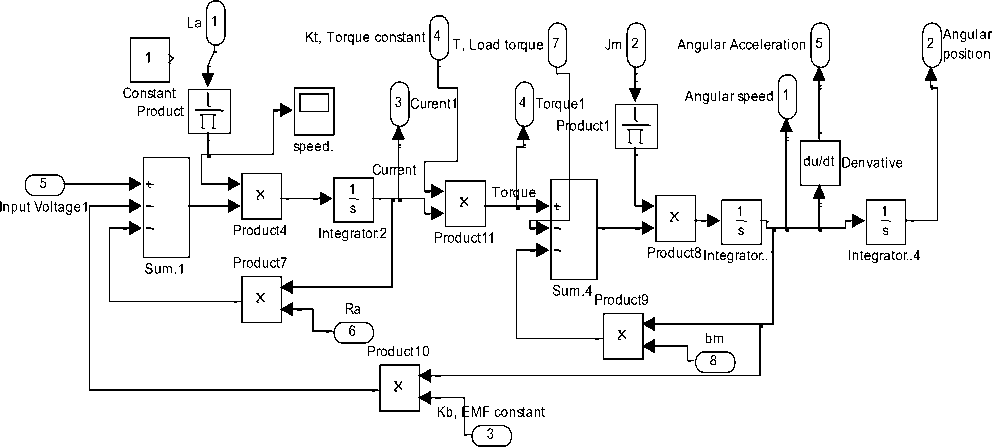
Fig. 2 (b)

Angular speed.

To File2

Fig. 2 (c)

Fig. 2(b)(c): Subsystem and function block model with its function block parameters window for DC motor performance verification and analysis [2]

To model, Simulate and analyze the open loop Robot arm system ,considering that the end-effector is a part of robot arm, The total equivalent inertia, J_equiv and total

equivalent damping, b equiv at the armature of the motor are given by:

b .  = b + b,  , equiv     m     Load

( N i

2

V N 2 7

J = J + J, „ equiv      m     Load

N l

N

V N 2

2

The geometry of the mechanical part determines the moment of inertia and damping ,To compute the total inertia, J_equiv , we first consider robot arm as thin rod of mass m , length ℓ , (so that m = ρ*ℓ*s ) , this rod is rotating around the axis which passes through its center and is perpendicular to the rod. The moment of inertia of the robot arm can be found by computing the following integral:

J Load = (8*(0.4) ^2)/12 = 0.106666666666667 kg.m²

Substituting, we obtain, J_equiv ,to be :

J equiv = J m + J load * (1/1)

J equiv = 0.02+0.107= 0.1267 kg·m²

l /2

J px²sdx = ps —1| l /2                       ³

l /2

l /2

Obtaining the total damping, b total , gives:

b equiv = b m + b load (1/1)

b equiv = 0.03 + 0.09 = 0.12 N.sec/m

m

= —s 2

l3 /8

sl

3

1= —ml

12

Calculating and substituting values in (14) gives:

In order to obtain total system transfer function, relating input voltage V in and Arm-Load output angular position θ Load , We Substitute values into transfer function given by (12) with gear ratio, n , gives:

_(J ) ₌ 9Load ( $ ) ₌___________________________ K, * П ____________________________

V in ⁽ $ )     { [ ( L a^Jequ^v $  ^{+ ( R} a^Jequ^v ^{+ b}equiv ^La ) $ 2 ^{+ ( R}a^bequiv ^{+ K} t^K b ) $ ] }

^G arm _ angle _ open ⁽ $ )

9Load ($ )

Vin(s)

0.0230.02913$3 + 0.1543$2 + 0.1205$

9 Load ( $ ) _ arm angle open ( $ )     T z /  \ __         Vin ( s )

0.023                                                   (4) $ ( s+4.342 )( s+0.9527 )

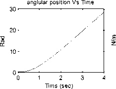
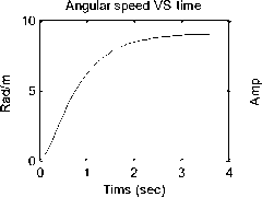
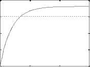
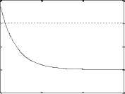
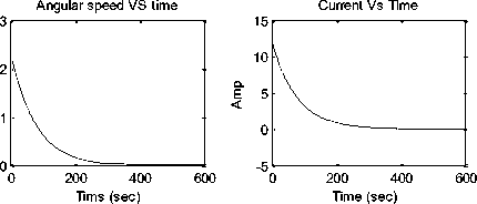
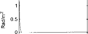
Defining the given DC motor's nominal values , gear ratio and arm parameters, and running any of both models ,We can analyze the performance of open loop Robot arm system and obtaining the response curves for step input voltage (0-12 volts), in terms of output Position/time, speed/time, Acceleration / time, Current/time and Torque/time, shown in Figure 3.

0.2

Torque Vs Time

0.4

0.3

0.1

123 Tims (sec)

Current Vs Time

Angular Accelaration VS time

Tims (sec)

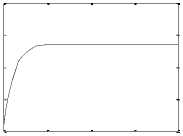
Fig. 3: Open loop DC motor system; Angular Position/time, Angular speed/time, Angular Acceleration / time, Current/time and Torque/time response curves for 12 V input

• III.    Control System Selection, Design and Analysis

A negative closed loop feedback control system with forward controller and corresponding Simulink model shown in Figure .4(a)(b) are to be used [3]. Our design goal is to design, model, simulate and analyze a control system so that a voltage input in the range of 0 to 12 volts corresponds linearly of an Robot arm output angle range of 0 to 180, that is to move the robot arm to the desired output angular position, θ L , corresponding to the applied input voltage, V in , with overshoot less than 5%, a settling time less than 2 second and zero steady state error. The error signal, e is the difference between the actual output robot arm position, θ L , and desired output robot arm position.

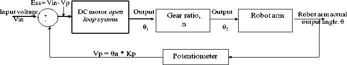
Fig. 4(a)

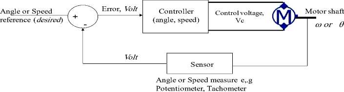
Fig. 4(b)

Fig. 4(a)(b): Two Block diagram representations of PMDC motor control [3]

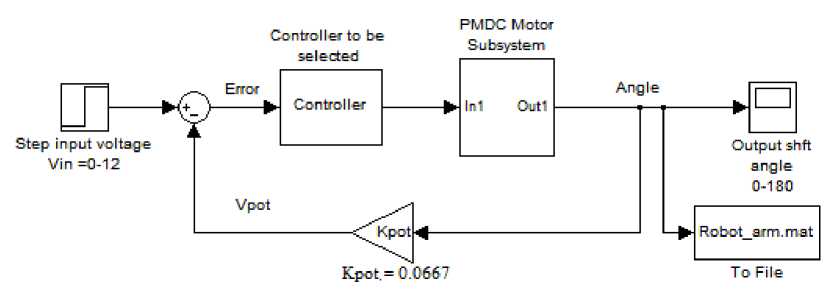
Fig. 4 (c): Preliminary Simulink models for negative feedback with forward compensation [3]

• 3.1    Sensor Modeling

• 3.2    Control Strategy Selection and Design

To calculate the error, we need to convert the actual output robot arm position, into voltage, V, then compare this voltage with the input voltage V_in, the difference is the error signal in volts. Potentiometer is a popular sensor used to measure the actual output robot (arm) position, θ L ,convert into corresponding volt, V p and then feeding back this value, the Potentiometer output is proportional to the actual robot arm position, θ L , this can be accomplished as follows: The output voltage of potentiometer is given by (5), in this equation: θ_L :The actual robot arm position. K_pot the potentiometer constant; It is equal to the ratio of the voltage change to the corresponding angle change, and given by Eq(5). Depending on maximum desired output arm angle, the potentiometer can be chosen, for our case V in = 0:12 , and output angle = 0:180 degrees, substituting, we have:

V = 0 * к p        L • pot

(Voltage change)pot   (Degree change)

( 180 - 0 )

= 0.0667 V / degree

The value (0.0667), means that each one input volt corresponds to 180/12= 15 output angle in radians , to obtain a desired output angular position of 180 , we need to apply 12 volts, to obtain an angular position of 90 we need to apply ( 90*0.0667= 6.0030 Volts).

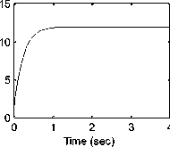
Running the Simulink model of the robot arm closed loop system without controller attached (K=1) shown in Figure 5(a), as well as the below MATLAB m.code , will return step response shown in Figure 5(b), the response curve shows that the arm system responds with a very huge value of settling time,(approximately TS=500 seconds) to reach steady state output angle of 180 degrees, that is not corresponding to the required design specifications. A controller is to be designed to meet desired specifications. In [3] different control strategies where applied to PMDC and it is found that, there are many motor control strategies that may be more or less appropriate to a specific type of application each has its advantages and disadvantages. The designer must select the best one for specific application , where when applying lag-controller to PMDC system, the system stability is increased, the settling time, Ts is reduced and steady state error is reduced, so called PD controller with deadbeat response, enables designer to satisfy most required design specifications smoothly and within a desired period of time and can be applied to meet the desired specification., applying internal model controller result in improving system's both dynamic and steady state performances, reducing overshoot, rise time and settling time as well as disturbance rejection, when applying PID controller to PMDC system, the system stability is increased, the settling time Ts is decreased and steady state error is almost eliminated, and so on. By proper selection the of the three PID gains, different characteristics of the motor response are controlled. To achieve a fast response to a step command with minimal overshoot and zero steady state error. We will, separately, apply these control strategies to our Robot arm system, and later to simplify and accelerate the whole process of robot arm system design in terms of designing the mechanical arm and gear parts as well as selection and designing the most suitable control strategy, a general model in the form of function block with its function block parameters will be built.

• >> Vin=12; Jm=0.02 ; Jm=0.1267;bm =0.12 ;Kt =0.023 ; Kb =0.023 ; Ra =1 ; La=0.23 ; TL = 0 ;Tl = TL ;n=1; M=8;desired_max_angle=180; Arm_Length =0.4 ;b_arm= 0.09;

Kpot =Vin/desired_max_angle; ;

J_equiv= Jm+((M* Arm_Length ^2)/12)*(1/n)^2;

b_equiv= bm + b_arm*(1/n)^2;

num_arm_open = [Kt*n];%[Kt*n*(180/pi)] den_arm_open=[La* J_equiv (Ra* J_equiv + La*

b_equiv) (Ra* b_equiv + Kt*Kb) 0];

disp(' Robot arm open loop transfer function , (Arm angle)/Volt')

Ga_arm_open=tf(num_arm_open,den_arm_open)

Ga_arm_closed=feedback(Ga_arm_open, Kpot/n),

step(12* Ga_arm_closed)

Current           Torque              Angular speed                    Arm angle- Radians

Arm angle feedbacK

Fig. 5(a): Simulink model of closed loop robot arm, with K=1

anglular position Vs Time

0      200     400     600

Torque Vs Time

0      200     400     600

K

GPID (s) = KP +    + KDs

s

_ KDs2 + KPs + K

K D

s2

0.3

0.2

0.1

-0.1

Tims (sec)

Tims (sec)

Angular Accelaration VS time

s

KK b—Ps + —

KDKD s

0       50      100      150

Tims (sec)

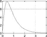
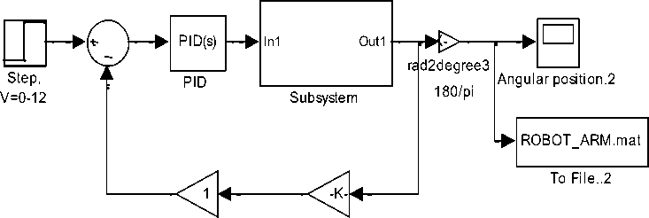
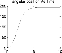
The Simulink model of closed loop robot arm, with DC motor, as subsystem and PID controller applied, is shown in Figure 6 (a). The response of this model is shown in Figure .6 (b). With optimal set of PID controller gains; KP, KI, KD, response curves still show the existence of steady state error (ess=0.0062) and overshoot of 0.024%. It is noted that the current can be controlled by adding and adjusting saturation block. The following MATLAB code can also be used to obtain step response

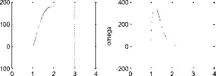
Fig. 5(b): Closed loop robot arm system step response Angular Position/time, Angular speed/time, Angular Acceleration / time, Current/time and Torque/time curves for 12 V input

>> Kp= 506.712827552343; Ki =

46.1017257705634; Kd= 562.448810124181

num_PID= [ Kd Kp Ki] ;

den_PID= [1 0];

G_PID= tf(num_PID, den_PID)

G_forward= series(G_PID, Ga_arm_open);

G_close_arm_PID = feedback(G_forward, Kpot/n) step(V*G_close_arm_PID) axis([0 8 0 200])

3.2.1 Controller Design Using PID Strategy:

PID controllers are commonly used to regulate the time-domain behavior of many different types of dynamic plants [6]. The transfer function of PID control is given by:

1/gear ratio Arm angle feedbacK2 =1/n2

Fig. 6 (a) Simulink model with PMDC motor subsystem and PID controller

Tims (sec)

Tims (sec)

Current Vs Time

_ (Kp + KDP) s + KPP=      s + P

= ( Kp + KDP) —

KPP

KP + KDP s + P

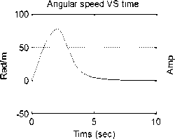
Fig. 6(a): Step response of closed loop robot arm, with DC motor, as subsystem and PID controller

Time (sec)

Now, let K_c = K_p + K_DP and z =

^K P ^P

K_p + K D P

we obtain the following approximated controller transfer function of PD controller , and called lead compensator:

G (s) = Kc

s + Zs + P

Lead compensator is a soft approximation of PD-controller, The PD controller, given by G PD (s) = K P + K D s , is not physically implementable, since it is not proper, and it would differentiate high frequency noise, thereby producing large swings in output. to avoid this, PD-controller is approximated to lead controller of the following form [13]:

If Z < P this controller is called a lead controller (or lead compensator). If Z > P : this controller is called a lag controller (or lag compensator) .The transfer function of lead compensator is given by:

Glead (s) = Kc

( s + Zo ) (s + Po )

Where: P > Z,

GpD (s ) - G Lead (s ) = KP + Kd

Ps

s + P

The Lag compensator is a soft approximation of PI controller, it is used to improve the steady state response, particularly, to reduce steady state error of the system, the reduction in the steady state error accomplished by adding equal numbers of poles and zeroes to a systems.

The larger the value of P , the better the lead controller approximates PD control, rearranging gives:

Gpi (s) -- Gag (s) = Kp + KI

s

Gbead (s) = Kp + Kd

Ps

s + P

KFs + K

s

_ Kp (s + P) + KDPs

= Kp

. ^    Kp >

s

Since PI controller by it self is unstable, we approximate the PI controller by introducing value of P o that is not zero but near zero; the smaller we make P o , the better this controller approximates the PI controller, and the approximation of PI controller will have the form:

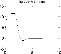
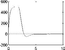
Where: Z o > P o , and Z o small numbers near zero and Z o =K I /K P , the lag compensator zero. P o : small number ,The smaller we make P o , the better this controller approximates the PI controller. The Simulink model of both Lead and Lag compensators is shown in Figure .7 (a). The step responses are shown in Figure .7(b).

G lag (^ ) = K

(^ + Zo ) (» + Po )

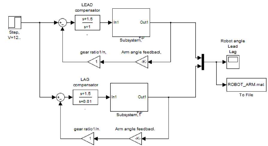
Fig. 7 (a): Simulink model of both Lead and Lag compensators

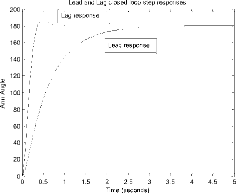
Fig. 7 (b): Position step response applying separately lead and lag compensators, step 12 volts, output 180 degree

• 3.4    Function Block for System Design and Analysis

• 3.4.1    PID Controller Function Block for Robot ARM Design and Analysis

To simplify and accelerate the whole process of Mechatronics robot arm system design in terms of designing mechanical parts; arm and gear , as well as selection and designing the most suitable control strategy, Two models in the form of function block with its function block parameters will be built, first simple using only PID controller and a second general model with most control strategies applied to Robot arm design and control.

A suggested Function Block model for robot arm design, controller selection, design and robot system analysis is shown in Figure .8 (b) , the function block subsystem is shown in Figure .8 (a). this model allows designer to apply Simulink PID controller block and its subsystem (P, PI, PD and PID) tuning capabilities and feature to select controller and analyze resulting robot arm response, by defining parameters of Robot arm subsystems (Arm, gears, and DC motor) selecting controller (PID), and running model, will result in speed/time and position/time curves shown in Figure .8(c) .

By changing the potentiometer constant, Kpot , the output angle range will change, Running this function block for the given robot arm, for an applied voltage of 0 to 12 volts and with Kpot =0.1333 will correspond linearly to an output arm angle of 0 to 90 , speed/time and position/time curves are shown in Figure .9(a), where Running this function block, for an applied voltage of 0 to 12 volts and with Kpot =0.2667 will correspond linearly to an output arm angle of 0 to 45 degrees, a 45 degrees position step response is shown in Figure .9(b)

Fig. 8 (a) Robot arm function block subsystem, using only PID Controller

Torque

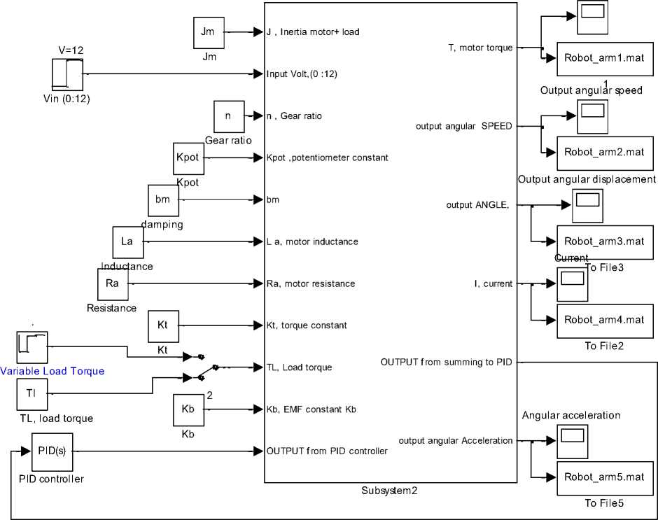
Fig. 8 (b) Function Block using PID for robot arm analysis and design

Output Angle                           Output speed

Time (seconds)                         Time (seconds)

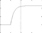
Fig. 8 (c) Speed/time and position/time response of function block using PID controller, K pot =0.066 , and Arm angular position θ = 180

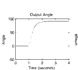
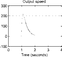
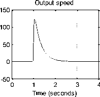
Fig. 9(a) Speed/time and position/time response of function block using PID controller, K pot 0.1333 , output angular position of θ = 180.

Output Angle

-20

Time (seconds)

3.4.2 A Proposed Function Block with Its Function Window Parameters, For Robot Arm Design, Controller Selection, Design and Verification

The suggested general function block is shown in Figure 10(b) based and subsystem in Figure 10(a), this model includes most control strategies applied to Robot arm design and control selection ,this model allow designer to define robot arm subsystems parameters, e.g. arm length, weight, gear ratio, damping factor, as well as to define electric motor parameter, e.g. V_in=12;J_m=0.02 . after defining all parameters, model allows using manual switch, select any control strategy , finally run the model and analyze response curves of a given robot arm system. the control strategies included in this model are, P, PI, PD, PID included in PID Simulink block, lead, lag compensator, PD with deadbeat, lead-integral controllers, model will return all the following response curves for any input from zero to 12 volts, Angular Position/time, Angular speed/time, Angular Acceleration / time, Current/time and Torque/time curves for 12 V input, this model, also, allows designer to use Simulink tuning capabilities of PID controller and its features. Switching model to PID controller, running simulation, will result in Arm position/time response curve shown in Figure .10 (c). This model can be modified to include other control strategies.

Fig. 9(b) Output Speed/time and position/time, (θ = 45), K pot =0.2667

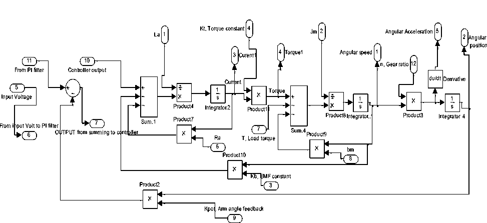
Fig. 10 (a) Robot arm function block subsystem

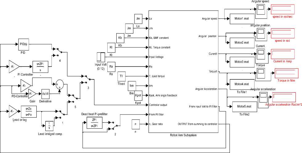
Fig. 10 (b) Function block with its function block parameters window for robot arm design, controller selection, design and verification

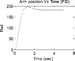
Fig. 10 (c) Arm position/time response of function block

• 3.5    A Proposed m.file for Robot ARM Research and Education

The following m.file can be used to return transfer functions, open loop and closed loop, with and without applying controller as well as corresponding responses and performance specifications.

clc, clear all, close all

Jm = input(' Enter Motor armature moment of inertia (Jm) :');

bm = input(' Enter damping constant of the the motor system (bm):');

Kb = input(' Enter ElectroMotive Force constant (Kb):');

Kt = input(' Enter Torque constant (Kt):');

Ra = input(' Enter electric resistance of the motor armature (ohms), (Ra):');

La =input(' Enter electric inductance of the motor armature ,Henry,(La) :');

V = input(' Enter applied input voltage Vin :');

V_max = input(' Enter maximum allowed voltage , V max :');

Angle_max = input( ' Enter maximum allowed angle for robot arm : ');

M= input(' Enter robot arm mass , M=');

Length = input(' Enter robot arm Length, L=');

b_arm= input(' Enter damping factor of robot arm, b_arm =');

n= input( 'Enter gear ratio n = ');

%obtaining open loop transfer functions of DC motor system and step response num1 = [1];

den1= [La ,Ra];

num2 = [1];

den2= [Jm ,bm];

A = conv( [La ,Ra], [Jm ,bm]);

TF1 =tf(Kt*n, A);

disp('DC motor open loop transfer function,

Speed/Volt: ')

Gv= feedback(TF1,Kt)

disp(' DC motor open loop transfer function,

Angle/Volt: ')

Ga=tf(1,[1,0] )*Gv subplot(4,2,1), step (V*Ga);

title(' Position step response of open loop DC motor system')

subplot(4,2,2)

step (V*Gv)

title(' velocity step response of open loop DC motor system')

%{ or based on open loop transfer function ,the following code can be used num = [Kt*n];

den=[La*Ja (Ra*Ja+Lm*bm) (Ra*bm+Kt*Kb) 0] disp(' Robot arm open loop transfer function,

Angle/Volt: ')

Ga =tf(num,den)

step (V*Ga)

%}

% obtaining open loop transfer functions of robot arm system and step response

J=((M* Length^2)/12)+Jm;

b= bm + b_arm;

num_arm_open = [Kt*n*(180/pi)];

den_arm_open=[La*J (Ra*J+La*b)

(Ra*bm+Kt*Kb) 0];

disp(' Robot arm open loop transfer function , (Arm angle)/Volt')

Ga_arm_open=tf(num_arm_open,den_arm_open) subplot(4,2,3)

step(V*Ga_arm_open);

title(' Position step response ,open loop arm system') subplot(4,2,4)

comet(step(V,Ga_arm_open))

title(' Position step response')

% Obtaining closed loop transfer functions of robot arm system and step response

Kpot=V_max /Angle_max; % potentiometer

G_close_arm= feedback(Ga_arm_open,(Kpot/n)) subplot(4,2,5), step(V*G_close_arm);

title(' closed loop position step response') subplot(4,2,6)

comet(step(V*G_close_arm))

title(' Robot arm Position step response') xlabel(' ')

• % Controller Design : PID Controller Kpro=input(' Enter Proportional gain Kp :'); Ki=input(' Enter Integral gain Ki :');

Kd=input(' Enter derivative gain Kd :'); num_PID=[Kd Kpro Ki] ;

den_PID=[ 0 1 0];

disp(' PID transfer function') G_PID=tf(num_PID,den_PID);

G_forward= series(G_PID, Ga_arm_open);

disp(' TF of Robot arm with PID controller, (Arm angle)/Volt')

G_close_arm_PID = feedback(G_forward, Kpot/n) % step(V*G_close_arm_PID) subplot(4,2,7)

step(G_close_arm_PID)

• IV. Conclusion

To simplify and accelerate the process of robot arm system design in terms of motor subsystem sizing, designing the mechanical subsystem, as well as selection and design of the most appropriate control strategy to achieve desired performance, two Simulink models first for open loop DC system motor selection and performance analysis and second for overall arm system performance analysis are proposed and tested.

Introduced models can be used to select and analyze the performance of open and closed loop systems and obtaining the Angular Position/time, Angular speed/time, Angular Acceleration / time, Current/time and Torque/time response curves for given input voltage; finally for research and education purposes, a MATLAB m.file is written, to return transfer functions, open loop and closed loop, with and without applying controller, as well as corresponding responses and performance specifications. Analyzing obtained response curves for different input voltage values, when different control strategies is applied, show the accuracy and applicability of derived models for research purposes in selection, performance analysis and control of mechatronics system requiring output position control.

center for researches.

engineering  studies  and technology