Modeling, Simulation and Dynamics Analysis Issues of Electric Motor, for Mechatronics Applications, Using Different Approaches and Verification by MATLAB/Simulink

Published Online April 2013 in MECS

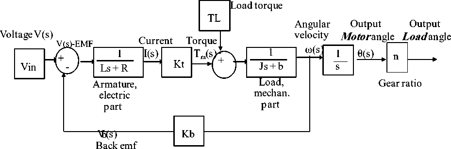
Mechatronic systems often use electric motors to drive their work loads, where electric motors are used to provide rotary or linear motion to a variety of electromechanical devices and servo systems [1]. Depending on application (e.g. robots, electric vehicles, low-to-medium power machine-tools etc.) and desired dynamic and steady state performances, as well as for motor's performance analysis, controller selection and design, it is of concern to derive mathematical models of electric DC motor, and built corresponding Simulink models, that can simplify and accelerate the process of modeling, simulation and dynamic analysis of DC motor motion control for mechatronics applications.

Motion control systems takes input voltage as actuator input, and outputs linear or rotational position/speed/ acceleration/ torque, the most used actuator for motion control systems is DC motors. A single joint robot arm is an application example of an electromechanical system used in industrial automation. Each degree of freedom (DOF) is a joint on Robot arm, where arm can rotate or translate, each DOF requires an actuator. When designing and building a robot arm it is required to have as few degrees of freedom allowed for given application, a single joint Robot arm is a system with one DOF. In industrial automation, the control of motion is a fundamental concern, putting an object in the correct place with the right amount of force and torque at the right time is essential for efficient manufacturing operation [2]. To simplify and accelerate the process of DC motors sizing and selection for different applications, We are to model, simulation and analyze the basic open loop DC motor system using different methods and verification by MATLAB/ Simulink, also to suggest MATLAB m.file and function block model for purposes of design and analysis.

• II.    Robot Arm System Characteristic

Single joint robot arm system consists of three parts (Fig. 1); arm, connected to actuator through gear train with gear ratio, n .

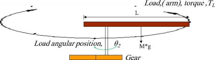
Motor angularposition, θ1

Motor torque ,Tm

Fig. 1: Schematic model of a single joint (one DOF) robot arm driven by an armature-controlled DC motor

The actuator used is a DC motor shown in Fig.2. DC motor turns electrical energy into mechanical energy and produces the torque required to move the load to the desired output position, θ_L , or rotate with the desired output angular speed, ω_L . The produced torque is exerted to accelerate the rotor and ultimately this mechanical power will be transmitted through a gear set to robot arm, therefore, part of the torque produced will cause a rotational acceleration of the rotor, depending on its inertia, J_m , and the other part of the energy will be dissipated in the bearings according to its viscous friction, b_m and the rotational speed.

• III.    Modeling the Electric Motor

DC motors (machines) consist of one set of a current carrying conductive coil, called an armature, inside another set of a current carrying conductive coils or a set of permanent magnets, called the stator. The input voltage can be applied to armature terminal (armature current controlled DC motor), or to carrying conductive coils terminals (field current controlled DC motor). This current will generate lines of flux around the armature and affect the lines of flux in the air gap between two coils, generating two magnetic fields, the interaction between these two magnetic fields (attract and repel one another) within the DC motor, results in a torque which tends to rotate the rotor (the rotor is the rotating member of the motor). As the rotor turns, the current in the windings is commutated to produce a continuous torque output resulting in motion.

DC machines are characterized by their versatility. By means of various combinations of shunt-, series-, and separately-excited field windings, they can be designed to display a wide variety of volt-ampere or speed-torque characteristics for both dynamic and steady-state operation. Because of the ease with which they can be controlled, systems of DC machines have been frequently used in many applications requiring a wide range of motor speeds and a precise output motor control [3, 4]. The selection of motor for a specific application is dependent on many factors, such as the intention of the application, correspondingly allowable variation in speed and torque and ease of control, etc.

The dynamic equations of DC motors can be derived, mainly based on the Newton’s law combined with the Kirchoff’s laws. The fundamental system of electromagnetic equations for any electric motor is given by [5,6]:

us = Ri + d—+jMkvs s ss dt           s

us = RRiR + d^R + j (^ - PbMm )V R > dtVs = Li. + L,iR

Vr  LRiR + LgiS

where : M the angular speed of rotating coordinate system (reference frame), Depending on motor construction (AC or DC), the method of the supply and the coordinate system (stationary or rotating with the rotor or stator flux) the above mentioned model becomes transformed to the desirable form [7], A designer can often make a linear approximation to a nonlinear system. Linear approximations simplify the analysis and design of a system and are used as long as the results yield a good approximation to reality [8].In modeling DC motors and in order to obtain a linear model, the hysteresis and the voltage drop across the motor brushes is neglected, and the motor input voltage may be applied to the field or armature terminals. In this paper we are most concerned with armature controlled and field controlled DC motor.

• 3.1    Modeling of the Armature Controlled PMDC Motor

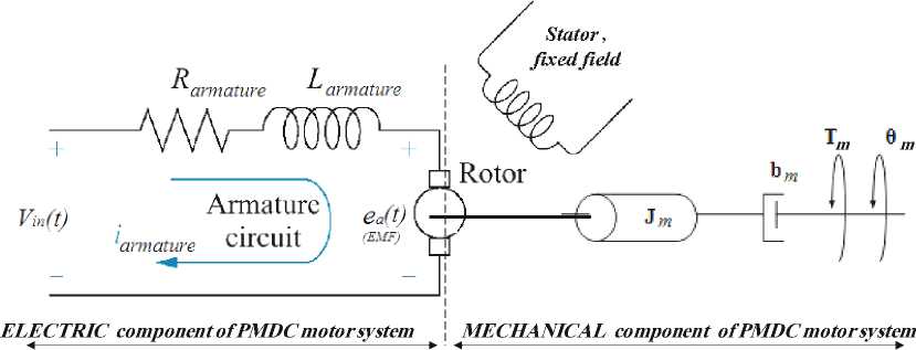
The Permanent Magnet DC (PMDC) motor is an example of electromechanical systems with electrical and mechanical components, a simplified equivalent representation the armature controlled DC motor's two components are shown in Fig.2(a).

ElectromechanicalPMDCmotorsystem

Fig. 2(a): Schematic of a simplified equivalent representation of the armature controlled DC motor's electromechanical components, (PMDC motor)

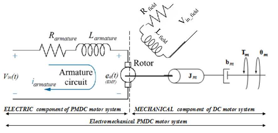
Fig. 2(b): Schematic of a simplified equivalent representation of the field controlled DC motor's electromechanical components

• 3.2    Modeling of Motor Dynamics, Approach I; The Basic Ideal, Linear, PMDC Motor Model

  • 3.2.1    Electrical Characteristics of PMDC Motor

Applying a voltage to motor coils produce a torque in the armature, the torque developed by the motor , T m is related to the armature current, i a by a torque constant, K_t and given by the following equation:

Motor Torque = T m = K_t* i a                ⁽ 2 )

equations describing mechanical characteristics can be derived; the sum of the torques must equal zero, we have:

u = J *a = J*d 2 9/dt 2

T e ^- T a ^{- T}_m^- T EMF = 0

Substituting the following values: T_e = K_t*i_a, T_a = J_m*-²9/dt² , and T_to= b_m*d9/dt , in open loop PMDC motor system without load attached, that is the change in T motor is zero, gives :

The back electromotive force, EMF voltage, e a is induced by the rotation of the armature windings in the fixed magnetic field, the polarity of EMF voltage acts in opposition to the current that produces the motion. The EMF is related to the motor shaft angular speed , to m by a linear relation given by:

К -T -I

K t ¹ T Load J m

г - 2 в '

V -t 2 )

Taking Laplace transform and rearranging, gives:

dO

ea (t) = Km dt

= K b ^ m

(3)

K t *I(s) - J m *s 2 9(s)— b m *S 9(S) = 0

K t I (s) = (J m s + b m ) s 9(s)              ^{( 7 )}

Where: K b : EMF constant. Based on the Newton’s law combined with the Kirchoff’s law, the mathematical model in the form of differential equations describing electric characteristics of the armature controlled PMDC motor can be derived, where the electrical equivalent of the armature circuit, can be described as an inductance, L in series with a resistance, R in series with an induced EMF voltage which opposes the voltage source. Applying Kirchoff’s law around the electrical loop by summing voltages throughout the R-L circuit gives:

У V = V - V - V - EMF = 0

in     R      L

Applying Ohm's law, substituting and rearranging, we get differential equation that describes the electrical characteristics of PMDC motor:

The electrical and mechanical PMDC motor two components are coupled to each other through an algebraic torque equation given by (1). In summary; a satisfactory PMDC motor equations that describes the electric and mechanical characteristics of a practical PMDC motor for many purposes is given by Eqs. (1), (2),(5) and (7).

• 3.3    Deriving PMDC Motor Open Loop System Transfer Functions

To derive the PMDC motor transfer function, we need to rearrange (6) describing electrical characteristics of PMDC, such that we have only I(s) on the right side, then substitute this value of I(s) in (7) describing PMDC mechanical characteristics, as follows:

V n = R a * i a ( t ) + L a f ^ Kb V -t )

- Q (t ) dt

Ia(s)

1

(LaS + Ra )

[Vi„ (S ) -Kb®(S )]

V

in

Г -i.> )   -d9

= ^Ra * i a ^{+ L}a l "T a l ⁺ K b™

V -t )       -t

(5)

The PMDC motor electric component transfer function relating armature current, and voltage, is given by:

Taking Laplace transform and rearranging, gives:

Y „ (s) = RJ(s) + L_as I(s) + K b s 9(s)

(L_as +R_a) I(s) = V_m(s) - K b s9(s)             ^{( 6 )}

Ia(s)

[Vin (s ) - Kb®(s )]

( L a s + R a )

• 3.2 .2 Mechanical characteristics of PMDC motor.

The torque, developed by motor, produces an angular velocity, to m = d9_m /-t, according to the inertia J and damping friction, b , of the motor and load. Performing the energy balance on the PMDC motor system the mathematical model in the form of differential

The PMDC motor Mechanical component transfer function in term of output torque and input rotor speed is given by:

^( s)[KtIa (s ) -Tl (s )]

( ^Jm s ^{+ b}m )

In case, no load attached, T_load =0, we have:

г-Д s)[KG (s )]

1

(J ms + bm )

Now, Substituting (8) in (7) , gives:

K t

1

( LaS + Ra )

[Vin (s) - KVAs)]

(11)

= Jms9( s) + bms0( s )

Rearranging (11), and knowing that the electrical and mechanical PMDC motor components are coupled to each other through an algebraic torque equation given by Eq. (1), we obtain the PMDC motor open loop transfer function without any load attached relating the input voltage, V_in(s), to the motor shaft output angle, θ m (s) , given by:

^Gangle ^{( s} ) = F Y)

K t

{ s [ ( L_os + R_o )( J s + b_m ) + KK . ] }

G ^ngle ( s ) =

9 s )

V in ( s )

K t

{ [ L a J m s 3 + ( N + bL. ) s ² + ( Rb + KK b ) s ] }

The PMDC motor open loop transfer function relating the input voltage, V in (s) , to the motor shaft output angular velocity, ω m (s) , given by:

G... (s ) =

аД s )

Vin(s)

K t

{[(Las + Ra )( Jms + bm ) + KKb ]}

(13)

G speed ( s ) =

® ( s )

V in ( s )

K t

{ [ L a J m s ² + ( R a J m + b m L a ) s + ( R a b m + KK b ) ] }

Here note that the transfer function G_angle ( s ) can be expressed as: G_angle ( s ) =G_speed ( s ) *(1/s) . This can be obtained using MATLAB, by the following, code:

>> G_angle = tf(1,[1,0] )* G_speed

Where: running tf(1,[1,0] ), will return 1/s

The open loop PMDC motor transfer function relating the torque developed by the motor, T m (s) and the output motor shaft angle θ m (s) , is obtained by rearranging Eq.(6), to give:

9m (s ) =       1Tm (s )  (Jms 2 + bms )

The open loop PMDC motor transfer function relating the armature voltage, V_in(s), to the armature current, I_a(s) , directly follows:

I a ( s )

V in ( s )

5 2 J R ,ь Y J Rb^K. ^

I L J J I L J L JM J a   m      am   aM

The armature, i a current can be found by rearranging the torque equation given by (1), rearranging and taking Laplace transform, gives:

Ia(s)

Tm(s) Kt

To find the transfer function of the PMDC motor, in terms of input voltage V in and output angular position θ m , we first substitute (3), and (16), in (5) and taking Laplace transform, this gives:

V ( A   ( ^La^s + ^Ra ) Tm ⁽ s       Ш A

V in ^{( s} ) =  ------------ ^{+ K}b^{s 9 ( s} )

^Kt                                    ( 17 )

The torque developed by the motor, T_m(s), in terms of output angle θ_m(s) , is given by (14), substituting in (17), and manipulating, gives:

( L_as + R_a ) ( J_ms ² + b_ms ) 9 ( s )

V, „ ( s ) = —---- a^m----- m ’    + K_bs 9 (s )

in                        _Kt                       b

Manipulating and Rearranging gives:

Vn (s) =

(Ra )(Jms 2 + bms ) Kt

+ Kbs

9( s)

[ ( L a s ^{+ R} a ) ( ^J m ^s "  ^{+ b} m s ) ^{+ K} t ^K b ^s ] ^{9 ( s} )

^V n ⁽ s ) = --------------------------------------

Kt

G ange ( s ) =

0 ( s )

V in ( s )

K t

{[ LaJmS 3 + (RaJm + bL ) S 2 + (Rabm + KK ) S ]} motor inductance, (La =0) , will result in the following simplified first order form of PMDC motor transfer function in terms input voltage, Vin(s) and output speed , ωm(s) given by:

Armature inductance, L_a is low compared to the armature resistance, R_a (discussed later). Neglecting motor inductance by assuming, ( L a =0 ), manipulating and gives:

G speed ^{( s} ) =

Vin(s)

^( s)

Vin(s)

K t R a J a

K t

{[( RaJm ) s +( Rabm )+ KKb ]}

1 L s +b u m V

Rearranging this first order equation into standard first order transfer function form, yields:

The torque is given by:

T= j d2θ/dt2 = J dω/dt

Also torque is given by (2), equating these two equations, separating armature current i_a , taking Laplace transform, gives:

Gspeed (s)   Vn (s)

K b K t

_   (Rab + KtKb)

RaJ

( R _a b + K t K b )

K t *i a = J m d²θ/dt²

(19)

I a ( S )

У2^ (s)

K t

Substituting (19) in (6), and rearranging gives:

У20 (s)(Las + Ra)       '  ' Vn (s) - ^6(s )

K _t

( JsW s')      JsWs'))

Ls —-- (-) + R —--- (-) + K_bs O (s ) = V„ (s )

a     a     bin

V       K t             K t )

angle

(s )==,___________ Kt___________.

V in ^(s )   [ L a J m s ⁺ R a J m s ^{+ K}t^Kb s ]

( 20)

(21)

KB

ts +1 s +1

A simplified first order form of PMDC motor transfer function in terms of output angle, can is also be obtained by substituting (La =0), and given by:

Gange (s ) =

e( s)Vin(s)

(22)

s

K t

RaJ

Eq.(12) can be simplified by substituting,( L a =0 ), to have any of the following two forms, where the second form given by (22) can be simplified to second order system, given by:

To write transfer function in terms of output speed ω , we rewrite the torque Eq.(19) in terms of output speed K_t*i_a= J_m dω /dt , and repeat previous steps.

• 3.6 Simplification of Open Loop PMDC Motor System Transfer Functions Models

Based on the fact that, the PMDC motor response is dominated by the slow mechanical time constant, where the electric time constant is much faster (e.g. ten times) than the mechanical time constant, this can motivate us to assume that the armature inductance, L a is low compared to the armature resistance, R a . neglecting

^Gangle ^{( s} ) =

0 ( s )

V in ( s )

K t

[ R.J„s2 + (Rabm + KtKb) s ]

K

s (s + a)

Also (20) by substituting,( L a =0 ), can be simplified to second order system relating input voltage and output angle, as well as equation relating input voltage and output speed, to be given by:

^Gangle ⁽ s ) =

0( s )Vin(s)

( 24)

K t

s (RaJmS + KtKb )

^Gspeed ⁽ s ) =

Vin(s)

( 25)

K t

(RaJmS + KtKb )

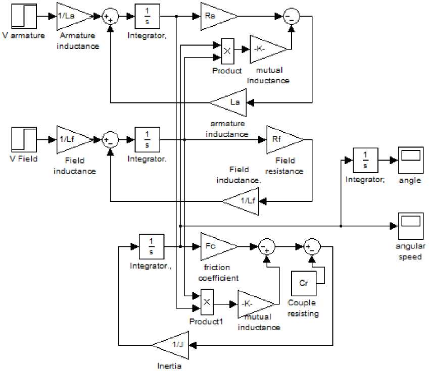
Mechanical control systems are supposed to operate with high accuracy and speed despite adverse effects of system nonlinearities and uncertainties. This robustness property is of great importance if the system is part of a robotic or servo system, which requires insensitivity to unmodeled dynamics [11,12]. The ideal simplified PMDC motor model rarely accurate compared with actual results and measurements, since note all factors are considered. To obtain the full system model, major mechanical and electrical nonlinearities such as saturation, coulomb friction and backlash must be included in the model. Here we will derive more an actual equations of PMDC motor, identifying all possible parameters, (actual simulink model is shown in Fig.7). Coulomb friction is a non-linear element in which forces tend to appose the motion of bodies in contact in mechanical systems, it acts as disturbance torque feedback for the mechanical system, Coulomb friction is considered to be a constant retarding force but is discontinuous over zero crossings, that is, when a DC motor reverses direction it must come to a stop at which point Coulomb friction drops to zero and then opposes the reversed direction. In effect Coulomb friction is constant when rotational velocity is not zero [3]. Introducing in Eq.(6) ,Coulomb friction and dead zone friction, where (T load =0) , we have:

K t *i a = T a + T_m + T load + T f

K t *I(s) - J_m *S 2 9(s)— b_m*s 9(s) - T f = 0

At steady state conditions, d/dt =0, gives :

K t *i_a = - b*to -T f

T f = K t *i_a - b*m                         ⁽ 26 )

IV. PMDC Motor Model Representation, Simulation and Analysis

Applying a voltage, V_in, to motor coils produce a torque in the armature. The produced torque produces an angular shaft velocity, to= dd/dt, according to the inertia J and viscous friction b , the armature will rotate at a speed and direction dependent on the applied voltage and polarity. Theoretically, as a result of applied voltage the motor shaft should continue to accelerate to a higher and higher speed unless there is a force that works in opposition to the applied voltage, this force is back electromotive force, EMF, e_b., where because the rotation of the PMDC motor's armature windings in the fixed magnetic field generates, EMF, that opposes the applied voltage. Using this we can build the block diagram model of the open loop PMDC motor system. The PMDC motor electric component transfer function relating input armature current, i_a and voltage V_in , is given by (9), the DC motor mechanical component transfer function relating output torque and input rotor speed is given by (10), also the electrical and mechanical PMDC motor components are coupled to each other through an algebraic torque equation given by (2), using these relations we can build the block diagram model of the open loop PMDC motor system shown in Fig.3 , block diagram model shows the feedback action in the open loop PMDC motor system, also shows that the electrical and mechanical PMDC motor components are coupled to each other through torque constant K t .

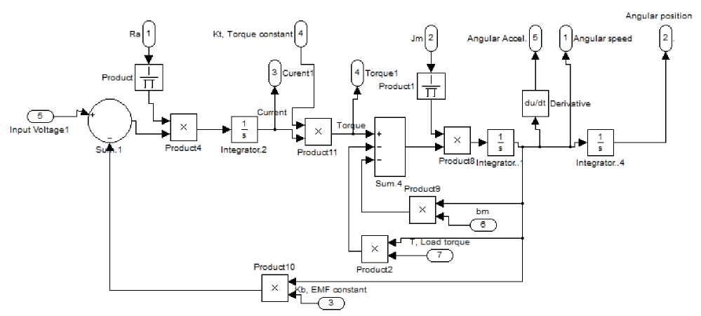
Fig. 3: The block diagram representation of open loop PMDC motor system

4.2 The Feedback Action of the Open Loop DC Motor System

Basically the DC motor is an open-loop system, to maintain a constant armature output angular velocity, (an increasing angle at constant value) the DC motor exhibits a speed feedback, this speed feedback is achieved by motor's built-in velocity feedback factor K_b , (The back-EMF constant), this closed loop is a accomplished as follows; If the load on the motor increases due to an increase in viscous friction, b m then the steady state angular velocity of the motor will reduce, this can be shown by equation K t *i a = b m *ω m . Rearranging, to obtain angular velocity we have, equation ω_m=K_t*i_a/b_m . This equation means an increase in viscous friction, b_m will result in reduction in steady state angular velocity of the motor. A reduction in steady state angular velocity produces a reduction in the back EMF, this is can be seen from (3). This change results in an increase in armature current which increases the developed torque, this is can be seen from (2) that closes the loop to maintain a constant armature output angular velocity.

‘ _d0_

• ¹    = dt " x ²

‘ d 2 0 _dm_K_t * i_Q b_m * m T_L ² = if⁼it = -j: j t "  Jm.

' ₌^dia _ ^Ra * i a ^Kb * ^m _ ^Vi„

• ³    dt       L a        L a      L a

Substituting state variables, for electric and mechanical part equations rearranging gives:

'

'

x ₂ —

' x ₃

d 0

— — x₉ dt

^“

bK mt

■x ^ Г       ^v

J m

J m

- T /

- K b x L

^“

^R a _x

L ³

+— V,

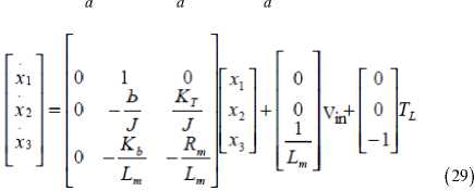
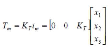
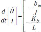
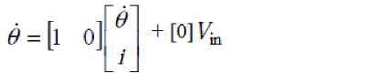
L

in

V. State Space Representation of PMDC Open Loop System

The state variables (along with the input functions) used in equations describing the dynamics of a system, provide the future state of the system. Mathematically, the state of the system is described by a set of first-order differential equation in terms of state variables. The state space model takes the following form [9]:

dx

= Ax + Bu dt y — CX + Du

Rearranging (5) and (6) to have the below two first order equations, relating the angular speed and armature current:

Looking at DC motor speed , as being the output, the following state space model obtained:

dm _ Kt * ia bm * m

-- —----- dt     Jm      Jm    Jm( din     Rn * i.  Kh *m V.

a           a     a        bin

-- —------ dt        La       La     La(

Looking at the DC motor output shaft position θ, and choosing the state variable to be the motor shaft output position θ m , velocity ω m and armature currents i a :

xx — 0

The state space models are the basis for building the simulink model of open loop DC model.

x ₂

d 0 dt

a

• VI. Simulation and Analysis of PMDC Motor Open Loop System Using Simulink

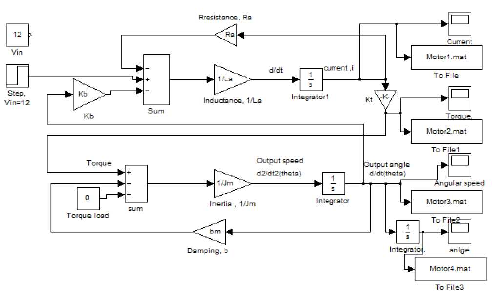
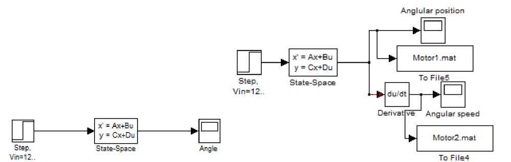
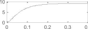
• 6.1    Simulation and analysis of PMDC motor open loop system based in state space representations given by (29) ,is shown in three suggested models in Fig.4(a)(b)(c), running any of these models will return Torque/time, Speed/time , Angle/time and Current/time curves for 12 V step input shown in Fig.9

  

  Fig. 4(a): simulink model based on state space representation

  
  
  
  
  

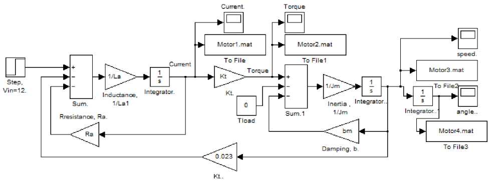
• 6.2    Simulation and analysis of PMDC motor open loop system based on transfer function model given by equations (12) and (13), is shown in Fig.5.

  

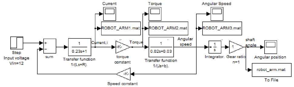
  Fig. 5: PMDC motor simulink model based on transfer function model given by (11)

  
  

  6.3 Block

  
  

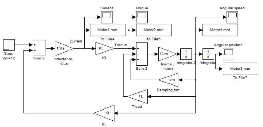
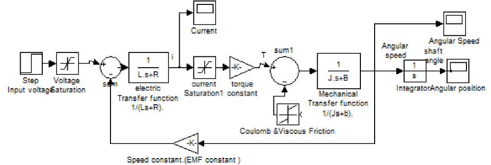
Using derived PMDC motor models, the following simulink models for Speed/time, Torque/time, Position/time and Current/time curves can be obtained, these curve can be used to evaluated, test and validate a given DC motor. Running any of the suggested simulink models with particular DC motor's parameters defined, will return curves shown in Fig.9, here notice that , depending on application, different equation was derived; simplified and accurate. The following nominal values for the various parameters of a PMDC motor used: Vin=12 Volts; Jm=0.02 kg·m²; bm =0.03;Kt =0.023 N-m/A; Kb =0.023 V-s/rad; Ra =1 Ohm ; La=0.23 Henry; TL = 0 ( no load attached).

Fig. 4(b): simulink model based on state space representation

Fig. 4(c): simulink model based on state space representation

mathematical model in simulink of PMDC motor given by equations (21) and (22), assuming La =0 , is shown in Fig. 6.

Fig. 6: Simulink model based on simplified mathematical model

Fig. 7: a suggested full block diagram model of PMDC motor open loop system with introduced saturation and coulomb friction

• 6.4    Suggested Function Blocks with Its Function Block Parameters Window

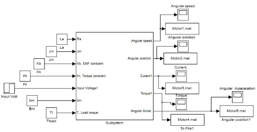
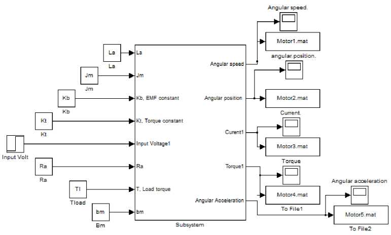
• 6.4.1    Simplified function block based on block diagram model, shown in Fig.8(a), is shown in Fig.8(b)(c), running this with nominal values, will return response curves shown in Fig. 9as well as angular acceleration/time curve.

• 6.4.2    Accurate function block based on simulink model, given in Fig.8(c), is shown in Fig.8(d). Running this with nominal values, will return response curves shown in Fig. 9, as well as angular acceleration/time curve, here note that the current/time curve will differ from that in Fig. 9(a) and is shown in Fig.9(b) , this is because of (La=0) simplification.

  

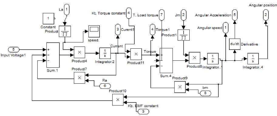
  Fig. 8(a): Simplified PMDC motor sub system

  
  
  

  Fig. 8(b): Simplified PMDC function block PMDC motor sub system

  
  
  
  
  

  Fig. 8(c): Simplified PMDC motor subsystem

  
  
  
  
  

  Fig. 8(d): Accurate function block with its parameters window for open loop DC motor performance verification and analysis

  
  

• 6.5    Modeling and Analysis Using MATLAB.

To simplify and accelerate the process of DC motors sizing and selection for different applications, the following two simplified and accurate a function blocks with its function block parameters windows are introduced below, these models can be used by defining parameters, in corresponding blocks or running m.file with these parameters defined and running the model, will result in corresponding Torque/time, speed/time , position/time and current/time curves for given step input volte.

The transfer function can be defined and entered in MATLAB in a number of different ways ; by defining the variables in the transfer function , that are: V in , R a , l a , K t , K b ,J m , b m in polynomial coefficient form, then defining numerator and denominator, or we can separately enter transfer functions describing mechanical and electric DC motor characteristics ,then combine them in series, and finally using MATLAB function feedback to create a feedback connection of two transfer functions, a program m.file can be written to simplify analysis process, the following m.file can be used to return the transfer function relations G angle (s), G speed (s), O m (s)Z T_m(s) , I_Q(s)/ V_m(s),simplified G speed (s), simplified G_angle(s) as well as their response to step input signal, shown in Fig. 10

clc, close all, clear all

Vin= 12;Jm=0.02 ;bm =0.03; Kt =0.023; Kb =0.023; Ra =1 ; La=0.23; TL= 0;

• % Jm = input(' Enter moment of inertia of the rotor, (Jm) =');

• % bm = input(' Enter damping constant of the mechanical system ,(bm)=');

% Kt = input(' Enter torque constant, Kt=');

% Kb = input(' Enter electromotive force constant, Kb=');

% Ra = input('Enter electric resistance of the motor armature (ohms), Ra =');

% La =input(' Enter electric inductance of the motor armature (Henry), La=');

% Vin = input(' Enter applied input voltage, Vin ='); num1 = [1];

den1= [La ,Ra];

num2 = [1];

den2= [Jm ,bm];

A = conv( [La ,Ra], [Jm ,bm]);

TF1 =tf(Kt, A);

disp('DC motor electric part Transfer function ,output current: ')

G_electric=tf(num1,den1)

disp('DC motor mechanical part Transfer function o,output speed: ')

G_mechanical=tf(num1,den2)

disp('DC motor system open loop Transfer function ,output angle ')

G_speed= feedback(TF1,Kb)

disp('DC motor system open loop Transfer function ,output speed ')

G_angle=tf(1,[1,0] )*G_speed disp('Transfer function relating torque developed by the motor , Tm(s) and shaft angle ?m(s),')

G_torque_angle=tf(1,[Jm,bm,0])

disp(' Transfer function relating torque developed by the motor , Tm(s) and shaft speed , ')

G_torque_speed=tf(1,[Jm,bm])

disp('Transfer function relating input Vin(s)and output current I(s) : ')

G_Current=tf([1/La,1/Jm],

[1,((Ra/La)+(bm/Jm)),((Ra*bm)/(La*Jm))+((Kb*Kt)/(L a*Jm)) ])

disp(' Simplified Transfer function relating input

Vin(s)and output angle: ')

G_angle_simpl=tf(Kt,[Ra*Jm,(Ra*bm + Kt*Kb),0])

disp(' Simplified Transfer function relating input

Vin(s)and output speed :')

G_speed_simpl=tf(Kt,[Ra*Jm,(Ra*bm + Kt*Kb)])

subplot(4,2,1), step(Vin*G_angle),title('Step response , output angle ')

subplot(4,2,2), step(Vin*G_speed),title('Step response , output speed ')

subplot(4,2,3), step(Vin*G_torque_angle),title('Step response , input motor torque output angle')

subplot(4,2,4),step(Vin*G_Current), title('Step response,Vin output current')

subplot(4,2,5),step(G_angle_simpl),title('Simplified response, output angle ')

subplot(4,2,6),step(Vin*G_speed_simpl),title('Simplif ied response, output speed ')

% state space num = Kt;

den_speed =

[(Jm*La),(Jm*Ra)+(La*bm),(Ra*bm)+(Kt*Kb )];

den_angle =

[(Jm*La),(Jm*Ra)+(La*bm),(Ra*bm)+(Kt*Kb ),0];

G_speed2=tf(num,den_speed);

G_anle2=tf(1,[1,0] )*G_speed2;

disp('State matrix, output angle: ')

[A1,B1,C1,D1]=tf2ss(num ,den_angle)

subplot(4,2,7), step(A1, B1, C1, D1), title('state space response,output angle')

disp('State matrix, output speed : ')

[A,B,C,D]=tf2ss(num ,den_speed)

subplot(4,2,8), step(Vin*A, Vin*B, Vin*C, Vin*D), title('state space response, output speed ')

% steady state calculations : % for velocity steady state value t=0:0.01:1000;

y=step(12* G_speed,t);

speed_steady_state_value=y(length(t));

fprintf(' Output steady state speed, OMEGA= %f rad/sec \n ',speed_steady_state_value)

% for angle steady state value y=step(12* G_angle,t);

angle_steady_state_value=y(length(t));

fprintf('Output steady state angle for given time range, THETA= %f radians \n ',angle_steady_state_value)

• VII. Modeling of Separately Excited DC Motor

• 7.1    Modeling of the field current controlled DC motor, with i_a (t) held constant

  A simplified equivalent representation of the field controlled DC motor's two components are shown in Fig.2(b). it consists of independent two circuits, armature circuit and field circuit, in which loads are connected to the armature circuit The voltage is applied to both to field and armature terminals, as shown , there are two currents, filed current, i_f(t) and armature current, i_a(t) in order to have linear system, one of these two currents most held constant. In the field current controlled DC motor, the armature current must maintained constant i a (t) = i a = constant , and the field current, i f varies with time ,t, this yields:

  The air-gap flux, Φ is proportional to the field current and given by:

  ф — K f * i f                               ( 30 )

  The back EMF voltage is given by:

  EMF = К* Ф * to m — V _[n - I a R a

  
  

  I ( ₅ ) — Vfy)                 ^{( 32 )}

  ^{fV 1}  ( L_fs + R_f )

  Where: L_f, stator inductance, R_f ,stator resistance

  The Mechanical characteristics of filed controlled DC motor; performing the energy balance on the DC motor system; the sum of the torques must equal zero, we have:

  ∑T = J *α = J*d²θ/dt²

  T m – T α – T ω = 0

  The motor torque is related to the load torque, by:

  T m –T ω = J*d²θ/dt²

  ^Km * i f ⁽ t ) - ^b m *s ⁶ ( s ) ^{— J}m *s² ^ ( s )

  
  

  Substituting (32) and rearranging, gives:

  
  

  The torque developed by the motor is related linearly to air-gap flux, Φ and the armature current i_a(t), and given by:

  
  

  Motor Torque = T _m = K 1 * ф *i_a (t )    ( 31 )

  
  

  Substituting (30) in (31), we have:

  
  

  T m — K 1 * K f *i_Q (t )* i f (t )

  
  

  K * V i_n_fi^{eid ( s}) _ ь y ( s ) — j 2 6 ( s ) ^{( 33 ) m} ( L_fs + R_f ) ^{m v 7 m v 7}

  Rearranging Eq.(33), the electrical and mechanical field current controlled DC motor components are coupled to each other through an algebraic the motor constant , K m , we obtain the transfer function relating input filed voltage V in_field (s), and motor output angle θ_m(s) , and given by:

  
  

  The armature current must maintained constant i_a(t) = i_a= constant, yields:

  
  

  ₌    6 ( s )   ₌          K m

  V in _filed ⁽ s )    s [ ( ^Lf s ⁺ R f )( Js ⁺ b ) ]

  
  

  T m = ( K 1 * K f *i_a )* i f (t ) = K _m * i f (t )

  Where K m : the motor constant. Based on the Newton’s law combined with the Kirchoff’s law, we obtain the mathematical model. Applying Kirchoff’s law, Ohm's law, and Laplace transform to the stator field yields mathematical model describing the electrical characteristics of field controlled DC motor and given by:

  
  

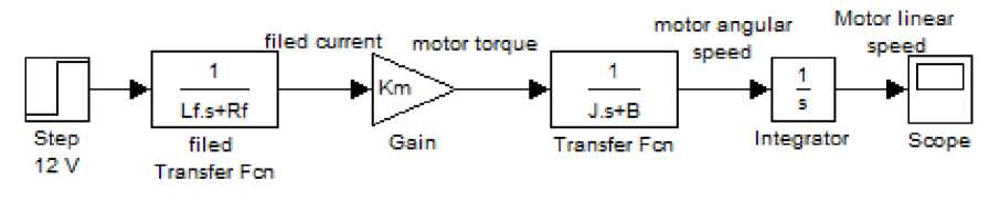
  The simulink model of the filed current controlled DC motor is shown in Fig. (11), here note that the armature controlled DC motor is in nature closed loop system, while filed current controlled DC motor is open loop.

  
  

  У V = V

  in _ field

  
  

  -V

  V _R

  
  

  field

  
  

  L _ field

  
  

  = 0

  
  

  Applying Ohm's law, substituting and rearranging, we get differential equation that describes the electrical characteristics, given by:

  
  

  7.2 Modeling of separately excited DC motor, with varying both i_a (t) and i f (t)

  Performing the energy balance on the DC motor system (Fig.2(b)); the sum of the torques must equal zero, we have:

  ∑T = J *α = J*d²θ/dt²

  T_e – T_α – T_ω - T_EMF = 0

  
  

V                        I di f ^{( t} )

• V.   г • 1л — R fi f + Lf\--------

• in _field      f f      f I ^

Te — K * i * i

Setting,          t s ^if , substituting, gives:

Taking Laplace transform and rearranging, gives:

V in_field (s) = (L f s +R f ) I f (s)

К      -T t     s     f      Load

J

m

k

dt

—

bm

Taking Laplace transform and rearranging, gives:

K*Us) * I f (s)- T_to ad - J m *S 2 9(s)— b m *S 9(s) = 0

K t *I a (s)* I j (s) - T load = (J m S + b m ) S 9(s)      ⁽ 3 ^{4 )}

K t * i f *

_ ( L _a S + R a ) _

[ V in ( S ) - K b * if * ^ ( S ) ]- T _loQ d

= ^Jm^S 2 ^ ^{( S} ) ^{+ b}m^{S 0 (S} )

( s )

[ K * I , ( S )* I f ( S ) - T l ( S ) ]

( ^Jm s ^{+ b}m )

[ K t * I _o ( S )* I f ( S ) - T_l ( S ) ]

® ( ^S ) =--------------

^{( J}m^{S + b}m )                   ( 35 )

Applying Kirchoff’s law around the field electrical loop by summing voltages throughout the R-L circuit gives:

Rearranging, the transfer function relating input armature voltage to output motor angular speed given by:

( S )

V ( s )

armature

K t I f

R a R f b

Г LJ A ₂ Г L_Q  J A L  ( K b V feld ) ^A

• -^ S +   + S + 1 +

[ Rb J   [ R_a  b J        RR)b

• \ ay      \ a      7     ^         a J ^

Vf = Rf * if (t ) + Lf

di f (t) A dt J

Taking Laplace transforms, rearranging to separate the field current, i f gives:

Vf = R f * I f (t ) + L f Sl _a

I_f ( s ) = 7--- V f ----7

^{( R}f ^{+ L}f^S )

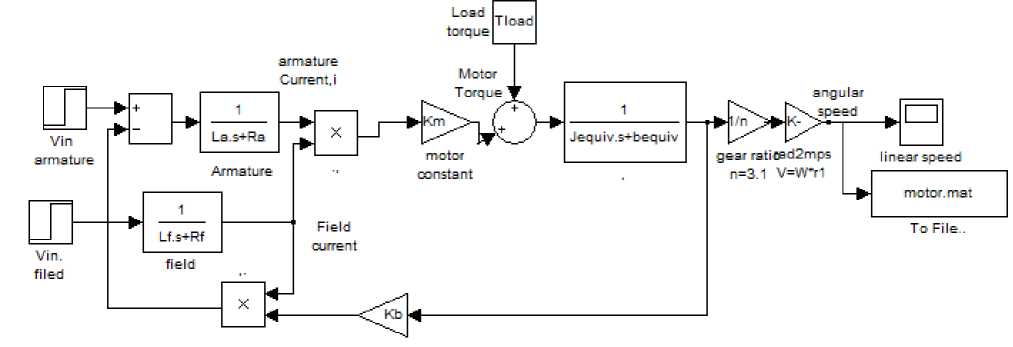
Applying Kirchoff’s law around the armature electrical loop by summing voltages throughout the R-L circuit, taking Laplace transform, gives:

Using these equation, the simulink model shown in Fig.12(a), of separately excited DC motor, can be built. Another modified from simulink model from [16] is shown in Fig.12(b), in this model the couple resisting, mutual inductance and coefficient of friction are introduced.

0.4

0.3

0.2

0.1

Torque Vs Time

У V = V - V - V - EMF = 0

in     R      L

Setting, EMF = K b * i f * d^ )/ ^dt , gives:

Tims (sec)

Current Vs Time 15

E

Time (sec)

V =R *z (t)^L a   aa    a

Г ^d i a (t )             dd0Q )

I + K b * i f *

I dt )                dt

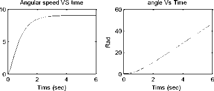
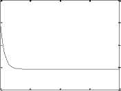
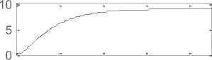
Fig. 9(a): Torque/time, Speed/time , Position/time and Current/time curves for 12 V step input

V in (s) = R a I(s) + L a S I(s) + K_b* i f * s 9(s)

Rearranging to separate the armature current, ia gives:

I a ( S ) =

( L..S + R _a )

[ V a ( S ) - K b

*i if

* to ( s ) ]

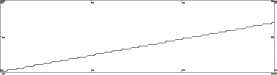
Angular acceleration VS time 8

0             5             10

Tims (sec)

Current VS time

12.1

11.9

11.8

11.7

0      5     10     15     20

Tims (sec)

Fig. 9(b): Angular acceleration/time curve, and simplified model current/time curve ,both for 12 V step input

Substituting in (34) .(35), gives:

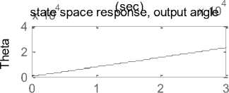
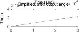
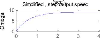
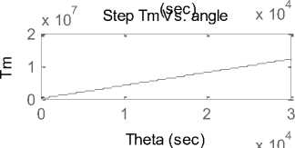
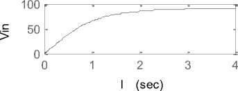
_{x 10}⁵    Step output Angle

Step output speed

state space resp(osnesce), output speed

Fig. 10: Response curves obtained by running suggested m.file

Step res poTnismee ,(VsiencV) s. current

Fig. 11: Simulink model of the filed current controlled DC motor

Fig. 12(a)

Armature resistance

Fig. 12(b)

Fig. 12(a)(b): Simulink model of separately excited DC motor

• VIII. Conclusion

To simplify and accelerate the process of selection, modeling, simulation and dynamic analysis of electric DC motors for specific mechatronics applications, this paper presents modeling, simulation and analysis of the basic open loop DC motor system, using different approaches and verification using MATLAB/simulink software, for different application, different mathematical and simulink models, as well as, a MATLAB m.file and function block models are derived , built and introduced , these models intended for research purposes as well as for the application in educational process, obtained response curves in terms of output torque/time, angular speed/time, angular position/time, angular acceleration/time and current/ time for 12V step input for used DC motor, reflect the accuracy and applicability of derived models for research purposes in selection, performance analysis and control of electric motors, as well as for research purposes and application in educational process.

• [1]    M. S. RUSU, and L. Grama, The Design of a DC Motor Speed Controller, Fascicle of Management and Tech. Eng., Vol. VII (XVII), 2008, pp. 10551060.

• [2]    Chun Htoo Aung, Khin Thandar Lwin, and Yin Mon Myint, Modeling Motion Control System for Motorized Robot Arm using MATLAB, World Academy of Science, Engineering and Technology 42 2008.

• [3]    Halila A., Étude des machines à courant continu, MS Thesis, University of LAVAL, (Text in French), May 2001.

• [4]    Capolino G. A., Cirrincione G., Cirrincione M., Henao H., Grisel R., Digital signal processing for electrical machines, International Conference on Electrical Machines and Power Electronics, Kusadasi (Turkey), pp.211-219, 2001.

• [5]    M.P.Kazmierkowski, H.Tunia "Automatic Control of Converter-Fed Drives", Warszawa 1994.

• [6]    R.D. Doncker, D.W.J. Pulle, and A. Veltman. Advanced Electri-cal Drives: Analysis, Modeling, Control. Springer, 2011.

• [7]    Grzegorz SIEKLUCKI,Analysis of the TransferFunction Models of Electric Drives with Controlled Voltage Source PRZEGL ˛ AD ELEKTROTECHNICZNY (Electrical Review), ISSN 0033-2097, R.88NR7a/2012.

• [8]    Richard C. Dorf and Robert H. Bishop. Modern Control Systems. Ninth Edition, Prentice-Hall Inc., New Jersey, 2001.

• [9]    Norman S. Nise, Control system engineering, sixth edition, John Wiley &  Sons, Inc, 2011.

• [10]    P. Wolm, X.Q. Chen, J.G. Chase, W. Pettigrew, C.E. Hann1, Analysis of a PM DC Motor Model for Application in Feedback Design for Electric Powered Mobility Vehicles.

• [11]    Slotine E, Li W. Applied nonlinear control. USA: Prentice Hall Inc.; 1991.

• [12]    Faber MN, Estimating the uncertainty in estimates of root mean square error of prediction: Application to determining the size of an adequate test set in multivariate calibration. Chemometr Intel Lab 1999;49(1):79–89.

• [13]    The MathWorks ( www.mathworks.com ), Control System Toolbox documentation Version V5.2 (R2009b).

• [14]    Katsuhiko Ogata, Modern control engineering, third edition, Prentice Hall, 1997.

• [15]    Boumediene Allaua, Abdellah Laoufi, Brahim GASBAOUI, Abdelfatah NASRI and Abdessalam Abdelrahmani Intelligent Controller Design for DC Motor Speed Control based on Fuzzy Logic-GeneticAlgorithmsOptimization. http://ljs.academic direct. org/ A13/090_102.htm

Appendix I: Table-Nomenclature

Symbol	Quantity	Unit
V, or Vin	The applied input voltage ,(Motor terminal voltage)	Volte, V
V in_field (s)	Input filed voltage	Volte, V
R a	Armature resistance,( terminal resistance)	Ohm ,Ω
R f	Stator resistance	Ohm ,Ω
L f	Stator inductance
L a	Armature inductance
Φ	Air-gap flux,
i a	Armature current	Ampere, A
I f	Field current
K t	Motor torque constant	N.m/A
K e	Motor back-electromotive force const.	V/(rad/s)
K m	The motor constant
ω m	Motor shaft angular velocity	rad/s
T m	Torque produced by the motor	N.m
J m	Motor armature moment of inertia	kg.m2
J total	Total inertia=Jm+Jload	kg.m2
L a	Armature inductance	Henry , H
b	Viscous damping, friction coefficient	N.m/rad.s
e a ,EMF :	The back electromotive force, EMF =K b dθ/dt	e a ,EMF :
θ m	Motor shaft output angular position	radians
ω m	Motor shaft output angular speed	rad/sec
V R = R*i	The voltage across the resistor	Voltage
V L =Ldi/dt	The voltage across the inductor	Voltage
T load	Torque of the mechanical load	T load
Tα	Torque du to rotational acceleration	Tα
Tω	Torque du to rotational velocity	Tω
T EMF	The electromagnetic torque.	TEMF