Modeling the Scheduling Problem of Identical Parallel Machines with Load Balancing by Time Petri Nets

Published Online December 2014 in MECS

Recent works in scheduling tend to classify problems and to find techniques to reduce their complexity by developing optimal and efficient algorithms. Among all classifications existing in the literature, Convay’s and Graham’s classifications are considered as the most used to encode such problems [1] and [2]. In [2], a clear separation is made between the three parts of the problem: task, resource and the objective to optimize. In these works, a task is an important element and it doesn’t carry about resources just using them without conflicts [3]. Nowadays with the technology advances, these traditional methods have proved to be inadequate because degrading system’s performances (inflexibility, lack of strategy in the adopted solutions for use resources, etc.) .

Petri nets are a formal tool for modeling and analyzing systems that exhibit behaviors such as competition, conflicts and the causal dependencies between events. They are appropriate to model and validate discrete event systems ( DES ). They are used for modeling concurrent systems such as Occam programs [4], the design of an automated production system [5] and recently in the protocol modeling for wireless sensor network [6].

Petri nets based approaches address the issue of flexibility of tasks and resources. The modeling power and analysis power of Petri nets theory can explore easily different aspects of the scheduling problem (behavioral and structural properties) and integrate factors ignored in previous works [7].

In scheduling related literature, Petri nets theory is applied in several fields. Ramamoorthy used graphical techniques to analyze the cyclical flow in automated production systems in order to represent the scheduling problem by cyclic Petri Nets [8]. Chrétienne provides a timed Petri nets based approach for cyclic generic scheduling problem [9]. Van Der Aalst exploits Petri nets to minimize the cycle time for planning repetitive problems [10]. Korbaa proposes a colored Petri nets based approach to model cyclic scheduling and to reduce the complexity analysis [11]. In [12], a Petri net-based model for scheduling problems with a branch and bound algorithm is proposed using dynamic branching strategy and resource-based lower bound. Other works on scheduling flexible manufacturing systems using Petri-nets and genetic algorithms are proposed in [13]; and colored Petri nets [14].

In these works, performance evaluation of the system is defined only in term of the task execution ordering without conflicts and resources sharing. This fact leads to a bad system performance.

In this paper, we extend classical methods by taking into account the load balancing aspect in the system, and ensuring an acceptable operating level. The method improves the conventional Petri nets based approaches by ensuring an economic resources using and achieving an acceptable state of the system. The modeled system can be analyzed to verify some properties like: finding a feasible scheduling, detecting conflict, eliminating redundancy, finding the lower/upper limit for the total execution time.

This work focuses on the formal modeling of identical parallel machines scheduling problem by using time Petri net and the formal validation of its properties by using TiNA tool. The preliminary results reveal that the obtained model load is bounded and adjusted among the resources.

The paper is structured as follows. Section 2 introduces some definitions on scheduling problem area with an illustrative example. In section 3, we introduce briefly the time Petri nets model. In section 4, we detail our method by explaining different mapping steps translating a scheduling problem into a time Petri net. The method is applied to an illustrative example and analyzed by TiNA tool. Finally we conclude with a conclusion and future prospects.

• II.    Scheduling Problem (SP)

Scheduling can be defined as the allocation of scares resources over time to perform a collection of tasks. It is concerned with finding the optimal one.

Scheduling techniques are used to answer questions that arise in production planning, project planning, computer control, manpower planning, cloud tasks scheduling, distributed simulations, etc. [15] and [16]. Many techniques have been developed for a variety of problems and classified by categories (single machine, parallel machine, flow job, job shop, etc.). To fix the terminology, we begin by defining the general scheduling problem.

Many problems fit into this definition. In essence, scheduling boils down to the allocation of resources to tasks over time. Some authors refer to resources as ‘machines’ or ‘processors’ and tasks are called ‘operations’ or ‘steps of a job’. Resources are used to process tasks. However, it is possible that the execution of a task requires more than one resource, i.e. a task is processed by a resource set. Moreover, there may be multiple resource sets that are able of processing a specific task. The processing time of a task is the time required to execute the task given a specific resource set. By adding precedence constraints it is possible to formulate requirements about the order in which the tasks have to be processed. We will assume that resources are always available, but we shall not necessarily assume the same for tasks. Each task may have a release time, i.e. the time at which the task becomes available for processing. A schedule is an allocation of resources to tasks over time and for each task it is specified when it is processed and which resources process it.

• A.    Definitions

Formally, an SP is defined as a triplet ( G T (T, C < ), R, C R ) where G T (T, C < ) is the tasks graph with:

• -    T: finite set of tasks T = {ff n with :

• -    s_i: starting time of the task execution T_i

• -    p_i: processing time of task T_i

• -    c_i: completion time of task T_i

• -    r i : release time of the task T i

• -    d i : due time

C < : precedence constraint (partial order relation on T×T).

T and C < make G T task-Graph.

Feasible scheduling: A scheduling is feasible if it satisfies the precedence constraints and resource availability constraint.

Objective function: The objective function is a metric that describes the quality of the solution based on specific objectives.

ϕ ∶ Π→ ℝ(1)

θ↦ԛ= ϕ(θ)(2)

Optimal scheduling: The optimal schedule is a feasible solution that optimizes the objective function on the state space.

θ∗ = Min ∈ ϕ(θ(3)

R : finite set of resources R= {R i } i.m with the maximum available amount m_i

C_R : resources constraint. It defines for each task, resource requirements with a_i j the necessary amount of resources R j for the execution of T i .

Scheduling: The scheduling of an instance of an SP is an application that associates to each task T i and its resource requirements, start time of its execution during p i .

θ ∶ Т ×R →ℝ (Т × R ) ↦ t

State space ( Π ): The state space is the set of all possible scheduling on T × R .

In the sequel we adopt the Graham’s notation [4]

<α|β|γ> for SP where:

• -    α represents the machine environment,

• -    ß represents the characteristics of tasks,

• -    γ is the objective function.

• B.    Illustrative Example.

The example illustrated by the Fig. 1 will be used in the sequel as a reference for our mapping method.

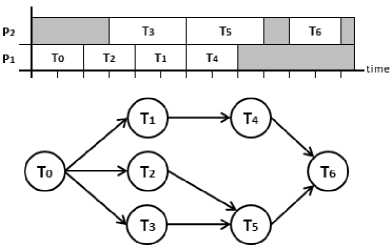
Fig.1. Tasks graph for a scheduling problem

According to Graham notation, Fig. 1 represents an instance of the SP , where the environment machine contains two identical parallel machines with precedence constraints and optimizing the total execution time as objective. The different elements of the SP are:

T = {T 0 , T 1 , T 2 , T 3 , T 4 , T 5 , T 6 }

P = {2, 2, 2, 3, 2, 3, 2}

< = {(T 0 , T 1 ), (T 0 , T 2 ), (T 0 , T 3 ), (T 1 , T 4 ), (T 2 , T 5 ), (T 3 , T 5 ), (T 4 , T 6 ), (T 5 , T 6 )}

R = {R 1 , R 2 } two instances of this kind of resources are available (processors).

C R : each task uses a unit of this resource for its execution.

Fig. 1 gives a possible solution to this instance, its configuration is:

Scheduling = {(T 0 , R 1 , 0), (T 1 , R 1 , 4), (T 2 , R 1 , 2), (T 3 , R 2 , 3), (T 4 , R 1 , 6), (T 5 , R 2 , 6), (T 6 , R 2 , 10)}.

• C.    Working hypotheses

In this study, a number of assumptions on the SP model are to consider:

• -    Simultaneous use of a resource by tasks is prohibited.

• -    Once launched, a transaction must complete without interruption.

• -    Lack of communication between resources and tasks.

• -    No duplication of tasks.

• -    Processing times are fixed and known in advance.

• -    Model used is parallel identical machines SP where resources are independent and having the same features. This model is classified by Graham as

  .

• III.    Time Petri Nets

Time Petri nets ( or TPN for short ) [17] and [18] are a convenient model for real time systems and communication protocols. TPN extend Petri nets by associating two values ( min, max ) of time ( temporal interval ) to each transition. The value min (min≥0), is the minimal time that must elapse, starting from the time at which transition t is enabled until this transition can fire and max (0≤max‹∞), denotes the maximum time during which transition t can be enabled without being fired. Time min and max , for transition t , are relative to the moment at which t is enabled. If transition t has been enabled at time α , then t cannot fire before α+min and must fire before or at time α+max , unless it is disabled before its firing of another transition.

We assume that the reader is familiar with the definitions and basic concepts of Petri nets [19].

• IV.    Modeling SP by Time Petri Nets

This section presents main steps of modeling SP by Petri nets. Entities of SP (task, resource, constraint) are associated to elements of Petri net model (place, transition, edge). Two main known translating methods are referenced in literature. These methods enable to map a SP into a Petri net model. The first method is due to Chrétienne and the second one is due to Van der Aalst. In both methods, translating process is made up of six steps: - Modeling tasks,

• -    Modeling precedence constraints,

• -    Modeling resources,

• -    Modeling constraints of available resources,

• -    Initial marking of time Petri net

• -    Synchronization mechanism.

Unfortunately in these methods, there is no way to control the policy of the resources used by the system. This fact is considered as the main drawback of such methods. For this reason, in this paper, we propose an extension of these traditional approaches by taking into account this fact.

• A. Scheduling Problem Modeling with Load Balancing

In previous methods there is no way to know how resources were used; also the interest is oriented only to tasks availability not for their loading. Our approach tries to combine the best of both previous methods by incorporating load balancing of resources. The main idea is to model separately each constraint, then separate the Petri net corresponding to the tasks graph from those corresponding to resources. Both Petri nets are connected in specific points through which communication is done. This approach allows us to adjust the load on resources resulting from the execution of tasks and therefore achieve a steady state system with a feasible scheduling. The method will be applied to the case study formed by identical parallel machines. Our mapping method proceeds in three main steps: mapping tasks graph into time Petri net task, mapping resources into time Petri net resources and finally connect these two generated nets [20] and [21].

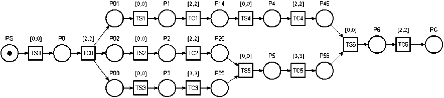
Fig.2. Tasks Time Petri net

Let SP = (G T (T, C < ), R, C R ) be an identical parallel • Mapping tasks graph machine scheduling problem.                                   G T (T, C < ) is transformed into tasks time Petri net

Step1 . Modeling tasks Ti (see Fig. 3 (a)).

• -    T Si start transition to launch T i

• -    P i associated place for T i

• -    T_Ci completion transition to end T_i.

• -    Create an arc from T_Si to P_i and another from P_i to T_CI

Step2 . Modeling the precedence constraint T i j by adding (see Fig. 3 (b)):

• -    P ij place associated with this constraint

• -    Create an arc from P ij to T SJ and another from T CI to

P ij

Step3 . Defining the initial marking

• -    All places are empty (initially no task is in execution).

Step4 . Modeling the synchronization mechanism

• -    The time is associated with completion transitions T_Ci and equal to p_i

  

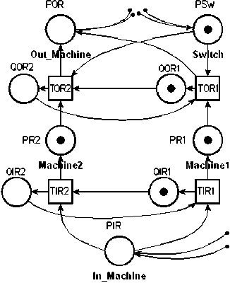
  Fig. 4. Resources Time Petri net

  
  

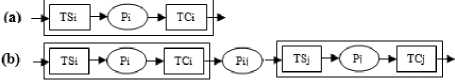
Fig.3. Tasks Time Petri net

In the resulting net, two specific places are added:

P_S : Start place to start the process. P_S is initialized with a token that passes through the rest of the net.

P_C : Completion place to end the process. The process stops when the token reaches the place P C .

By applying the mapping process to the SP illustrated by the Fig. 1, we obtain the tasks time Petri net represented by the Fig. 2. This part of solution illustrates a task graph side as a time Petri net node starting by task start transition. The place having a token represents the task processing and the task end transition represents the task delay. When the task finishes then delivers its outputs to the next step. The overall process starts with token on its first place PS and ends when the last transition PC expires it’s waiting time as execution of the last task in the task graph.

• •    Mapping resources

Resources are translated into Resources Petri Net.

Step1 . Modeling Input / Output Resources:

• -    R IP , R OP , P SW , Input/ Output / Switch place.

Step2 . Modeling resource R j is achieved by introducing:

• -    P RJ place

• -    Q_IR j , Q_OR j place points of entry / exit non-reentrancy be associated with Rj

• -    T_IR j , T_OR j transitions input / output of R j

• -    (P IR , T IRj ) (T ORj , P OR ) arcs are connected to the outside

• -    (T ORj-1 Q ORj ) (T IRj-1 Q IRj ) arcs connecting the preceding and following resources

Step3 . Defining the initial marking

• -    P RJ contains m tokens.

By applying these steps to SP of Fig. 1, we obtain the resource time Petri net illustrated by the Fig. 4.

• •    Connection of Tasks time Petri Net and Resources time Petri Net

Before the connection we model resource constraints and allocation of resources to tasks.

• - ( P OR , T Si ): Resource application.

• -    (T Si , P SW ): Notification of use of the resource.

• -    (T CI P IR ): Release of the resource.

Connection of tasks time Petri net (Fig. 2) and resources Petri net (Fig. 4) forms a time Petri net illustrated by the Fig. 5.

When the task is ready to run it consumes available resources modeled by the place P OR . Then, this task generates a token on the place P SW meaning that the next resource is ready to be consumed. The load distribution is ensured by the fact that each resource can be fairly used. When the place P SW will be marked up it goes out to the next resource that will put the token in the place P or (see Fig. 5). This process is repeated while exist enough resources to satisfy requests made by tasks. In other words, we expect the release of used resources. When a task completes then it releases the possessed resource. By recovering this resource, the place P_IR gives the control to the next resource.

This solution respects two principles; the first one using the resources in round robin fashion and the second concerns the availability of the resource for task execution. In this situation, the execution is blocked until a resources is released (become available) then it will be allocated to one of the waiting tasks. After this we will pass turn token to the next resources as marked for allocating next time.

• B. Properties Analysis

The analysis of time Petri net illustrated by the Fig. 5 is performed using the TiNA tool software version 8.0 (. The analysis has shown that the network has good properties. Fig. 6 summarizes some analytical results given by Net Control Draw of TiNA tool. It is possible to analyze all firing sequences of a time Petri net corresponding to a scheduling problem. Each firing transitions sequence starting from initial marking to final marking corresponds to a feasible scheduling. Transition sequences belonging to time Petri net given by Fig. 5 define the using of resources by the tasks. A transition sequence from the initial place PS to final place PC models ordered execution of tasks and ordered use of resources.

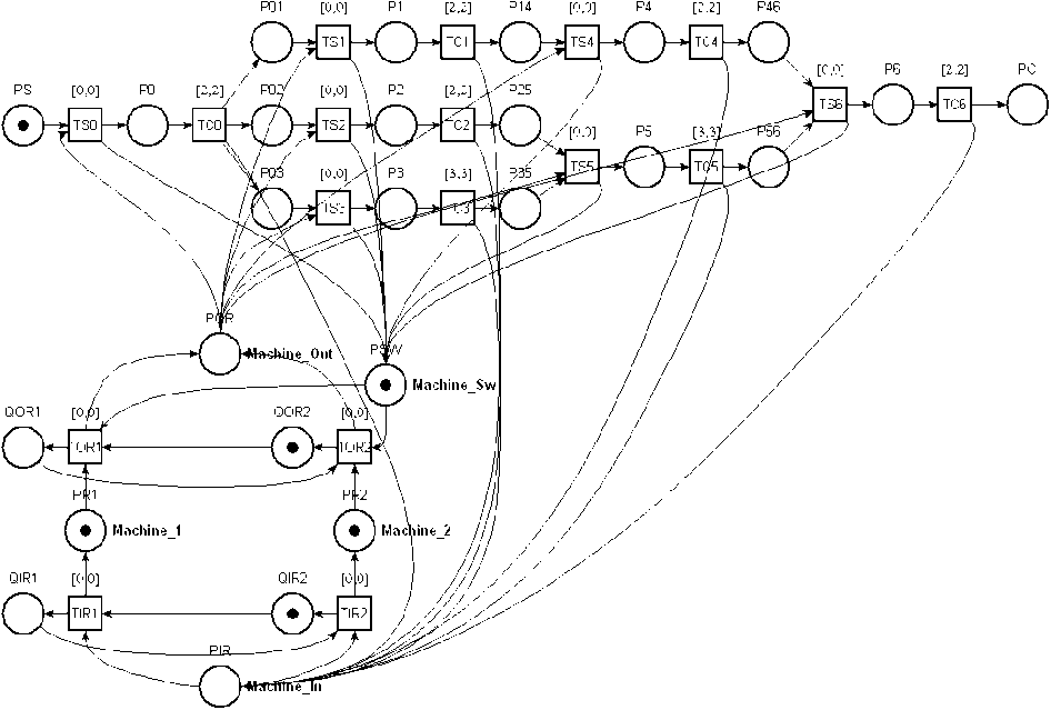
Fig. 5. Time Petri net of SP

, Used-Ressource,

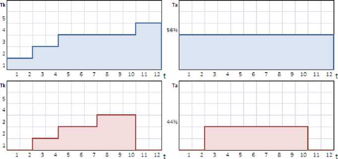
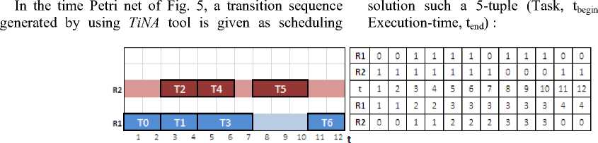
Fig. 6. Gant chart for resources utilization

TRACE = TOR1@0.0 TS0@0.0 TOR2@0.0 TC0@2.0 TS2@0.0 TIR1@0.0 TOR1@0.0 TS1@0.0 TC2@2.0 TIR2@0.0 TC1@0.0 TOR2@0.0 TS4@0.0 TIR1@0.0 TOR1@0.0 TS3@0.0 TC4@2.0 TIR2@0.0

TOR2@0.0 TC3@1.0 TS5@0.0 TIR1@0.0 TOR1@0.0

TC5@3.0 TS6@0.0 TIR2@0.0 TOR2@0.0 TC6@2.0

TIR1@0.0

SOLUTION = {(T0, 0, R1, 2, 2), (T1, 2, R1, 2, 4), (T2, 2, R2, 2, 4), (T3, 4, R1, 3, 7), (T4, 4, R2, 2, 6), (T5, 6, R2, 3, 10), (T6, 10, R1, 2, 12)}

Resources utilization of R1 and R2 are 75% and 58% respectively with a load average of 56% to R1 and 44% to R2 (number of assigned tasks), maximal difference between loading of R1 and loading of R2 is equal to one task. For our example above, the obtained solution has an acceptable balanced load among the whole system. This situation allows us to get good level of performance using the available resources. The classical methods do not permit to know such information because there is no way to save which resource executes which task. Fig. 6 shows the solution of the previous example, the load of each resource and the average load of using them.

Many of the scheduling problem solution can be modeled as reachability problems. In [22], the authors propose a constraint programming based approach to address the reachability problem. The authors use an incremental methodology based on linearization techniques to translate the reachability graph of a timed Petri net into a mathematical programming model.

An enumerative method exists in order to exhaustively validate the behavior of time Petri net. This technique is related to the reachability analysis method for usual Petri nets and allows one to formally verify time dependent systems. The TiNA tool uses the enumerative method and is applied to the verification of time Petri net model of SP illustrated by the Fig. 5. The analyze reveals that our SP has good properties as summarized in Fig. 7.

REACHABILITY ANALYSIS -...................-...................

bounded

174 marking(s), 318 tiansition(s)

MARKINGS:

0PR1 PR2PS PSWQIR2Q0R2

• 1    : POR PR2PS QIR2Q0R1

• 2    : PO PR2 PSWQIR2Q0R1

• 3 : P01 P02 P03 PIR PR2 PSW QIR2 QOR1

• 4    : P01 P02 P03 PR1 PR2 PSW QIR1 QOR1

• 5    : P01 P02 P03 POR PR1 QIR1 Q0R2

• 6    : P02 РОЗ P1 PR1 PSW QIR1 QOR2

• 7 : P02 РОЗ P14 PIR PR1 PSW QIR1 QOR2

• 8    : P02 РОЗ P14 PR1 PR2 PSW QIR2 QOR2

• 9    : P02 РОЗ P14 POR PR2 QIR2 QOR1

• Fig. 7. Analysis Results given by TiNA

The reachability graph shows all accessible states. In the context of our case study by time Petri nets, the reachability graph represents a spanning tree of all possible paths for task execution. Based on the properties of such graph, we can determine not accessible states, all terminal states (leaves of the tree), etc. If one of these leaves matches a final task in the task graph then we find a critical path that shows the longest sequence of tasks execution in this graph.

After launching the simulation, we will save its trace. By analyzing it, we will depict the most important features of this modeling method. Fig. 7 depicts that time Petri net of Fig. 5 is bounded and the reachability graph (state classes’ graph) contains 174 markings (state classes) and 318 transitions. The trace generated by TiNA simulator shows that the obtained solution has 12 units length, this means that the optimal solution has a Makespan C_max<= 12 units for this instance of problem.

So, based on this result, we can fix the parameters of other algorithms to get this optimal solution.

• V. Conclusion and Future Perspectives

In this paper we have proposed a new approach to mapping a scheduling problem into a time Petri net. This work extends previous works by taking into consideration the load balancing factor. Our mapping method is applied to specific class of SP ( identical parallel machines ). The method is based in a clear separation between main parts of a SP : tasks graph and resource constraints. Both parts are translated independently into a time Petri net. The resources time Petri net can be apportioned equally (resource use policy) serving requests from the first time Petri net ( tasks Petri net ). The transformation of a SP into a time Petri net allows us to analyze properties as: detecting resources conflicts, search of feasible scheduling, determining bound inf/sup of global run time, load balancing, etc. This validation can be done by software TiNA tool. Actually, as future prospects, we plan to extend our method to other classes of SP as no identical heterogeneous parallel machines.

Acknowledgment

This work was supported in part by the Industrial Computing and Networking Laboratory of Oran University.