Моделирование распределения температуры электронов в области F2 высокоширотной ионосферы для условий зимнего солнцестояния

Mathematical modeling of the high-latitude ionosphere involves the numerical solution of hydrodynamic equations with due regard to the mismatch between geographic and geomagnetic poles. This is due to the fact that the large-scale structure of the high-latitude ionosphere is controlled by universal time (UT-control). Moreover, the mismatch should also affect the thermal regime of the high-latitude ionosphere. Therefore, when calculating spatial-temporal distribution of temperature of charged particles, a need arises to make allowance for the UT-control. The numerical simulation of thermal regime of the high-latitude ionosphere, which is based on the Lagrange approach, has been described in a number of papers [Schunk et al., 1986.; Klimenko et al., 1991; Mingalev et al., 2002], which analyze, in particular, causes for the formation of “hot spots” ( T e ≥5000 K) [Koffman, 1984].

In this paper, we study the mismatch between the geographic and geomagnetic poles in the distribution of electron temperature in the F2 region of the high-latitude ionosphere in winter, using the Euler approach. This study relies on a three-dimensional model of the high-latitude ionosphere in Euler variables, which accounts for the thermal regime of the ionosphere. We make allowance for the mismatch between the geographic and geomagnetic poles, which produces the longitudinal effect in electron density distribution [Kolesnik et al., 1983]. We report the results of calculations of the spatial-temporal distribution of electron temperature in the F2 region for 05 and 17 UT when the Eastern and Western hemispheres are on the illuminated side. The calculations are made for winter solstice conditions, minimum solar activity, and moderate geomagnetic activity.

MODEL OF THE HIGH-LATITUDE IONOSPHERE

The model of the high-latitude ionosphere enables us to describe ionospheric plasma at a height range 120 ÷ 500 km. It has the following set of parameters: densities of electrons n e , ions n (O⁺), and basic neutral particles n (O), n (O 2 ), n (N 2 ), as well as temperatures of electrons T e , ions T i , and neutral particles T n . In the height range considered, we can take the condition of plasma quasi-neutrality n (O⁺) = n e . We use a spherical geographic coordinate system: r is a radius, θ is a colatitude, φ is a longitude. The model equations are written in the form presented in [Kolesnik et al., 1993].

To determine the O+ ion density, we use the continuity equation for O+:

( ) = q ( O ⁺)^- l ( Olf n ( O ⁺) ur ]- „ 1 a te^[ n ( O ⁺) u » ^sin9 ]+^[ n ( O ⁺) ^u ф ]} ^{,   (1)}

d t                       d r^L ' ^J R sin 9 d 9 ^{L J} dф^{L          J}

E where q (O+) and l (O+) are rates of local formation and losses of O+, cm–3·s –1; uir, uiθ , and uiφ are components of the velocity vector of O+, cm·s–1; RE is the Earth radius.

Electron temperature distribution in the high-latitude ionosphere is calculated from the thermal conductivity equation for electrons:

d T e      d T e    U e9 d T e      U     d T e       2 _  d U e,       1 d z . _x 1     ^d U _; .

+ u11T1(u sin 9) + dt    er dr   RE d9   REsin9 дф      3e^dr   REsin9 d9v e9     ’  REsin9 дф

• 2    [ H 22 d Г, d T ) К d( HH . Jd T

  ' ,---( ^QeX ^{+ Q} ep - ^L en - ^L ei ) ,

  3 kn _e

  
  
  
  

+--г—I К _e—- 1 +---e--1  ^y r sin 9 I —-

• 3    kn _e ^ H ² d r (   d r J R Esin 9 d 9 ( H ²       ) d r

where u e r , u eθ , and u eφ are components of electron velocity vector, cm^s·s^–1; λ e is the heat transfer coefficient of electrons; Q eλ is the rate of local photoelectron heating of electrons, erg cm^–3·s^–1; Q ep is the rate of charged-particle heating of electrons, erg cm^–3·s^–1; L en and L ei are rates of local heating or cooling of electrons due to elastic and inelastic collisions with neutral particles and ions respectively, erg cm^–3·s^–1.

The ion temperature is found from the thermal conductivity equation for ions:

д T     д T  u _i6 д T     u -ф    д T

+ u 11

д t    ^{1 r} д r   R E д 6    R E sin6 д ф

2 t +

3 ¹ д r

д u -i,

1 д

H r д

3 kn j H ² д r

д T ) Z д HH + i ⁶

д r ) R_v sin 6 д 6 1 H ² E

д r

R sin 6 д 6 E

( u _i6 sin 6 ) +

1 ^д u -ф

R E sin6 д ф

+

д T i

^ д T 2 , sin 6 —- +--(Q — L + Q-d), )д r J   3 kn i (                )

д r

where λ i is the heat transfer coefficient of ions; Q ie , L in are rates of local heating or cooling of ions O⁺ due to interaction with electrons and neutral particles, erg cm^–3·s^-1; Q id is the rate of O⁺ heating by electric fields and thermospheric winds respectively, erg cm^–3·s^–1.

The equations for the components of O+ velocity vector are defined as

1 ^{д n} ( O ⁺) 1 д T p 1 n ( O ⁺) д r T p д r H _p

sin² 1 + —

R

1 ^{д n} ( ^{O +}) £ д T n ( O ⁺) д 6 T 17

cos I sin I ^ +

cE

+--- cos I + u„„

H         nθ

sin I cos I ;

1 д n ( O ⁺) £ д T p 1 n ( O ⁺) д r     T p д r H _p

1 д n ( O ⁺)

sin I cos I +——   , .

R e [ n ( O ⁺)    д 6

1 д T +

T д r

1 r cos I ^ —

--^- sin I + u n ₆ cos² 1 ;

cEφ u„„ =----cosec1, iφ    H where Tp = Te + Ti; Hp = kTi/(m(O+)g); k is the Boltzmann constant, erg·K–1; g is the gravitational acceleration, cm·s–2; Eθ and Eφ are the meridional and zonal electric field components respectively, V·cm–1 ; H is the geomagnetic field strength, Oe; Da is the ambipolar diffusion coefficient, cm2·s–1; I is the geomagnetic inclination, deg; unθ is the meridional component of neutral gas velocity, cm·s–1. When deriving (4), we drop the vertical electric field component Er as in [Stubbe, 1970]. To fulfill the quasi-neutrality condition, we put electron and ion velocities equal to (йе = z/i). We ignore the zonal thermospheric wind velocity component in this article because it is insignificant (directed across geomagnetic field lines) as compared to the meridional one.

We focus on the electron temperature and therefore use expressions for rates of heating and cooling of electron gas at heights of the F2 region. In the illuminated part of the high-latitude ionosphere, the main source of thermal electron heating is photoelectrons Q _eλ formed during photoionization, whereas in the auroral oval it is secondary electrons formed during corpuscular ionization Q ep . Respective heating rates are specified according to [Krinberg et al., 1984]:

Q eλ =ε q ph ,

Qep=εqcorp, where qph is the rate of ion formation due to shortwave solar radiation; qcorp. is the corpuscular ionization rate;

ε=0.16

г

9 + lg

-n e_ I Z N n )

1.602 - 10 ^{- 12},erg.

Thus, it follows that the regions of photoionization and photoelectron heating coincide. The rate of electron gas cooling due to elastic collisions with O+ has the form [Banks et al., 1973]

,    n (O+)                                ,

L_d = 7.7 - 10 ^{- 6} nT ^{- 3/2} ( T - T ) x \ \ 1.602 - 10 - ¹², erg^cm^-3^s^-1 ei e e \ e i; m ( o + )

where M (O⁺) is the ionic mass O⁺. Cooling rates of the electron gas when interacting with neutral particles are set in accordance with [Schunk et al., 1978]. Temperature and density of neutral components are calculated by the thermospheric model NRLEMSIS-00 [Picone et al., 2002]. The electric field of magnetospheric convection is specified by Heppner’s model “A” [Heppner, 1977]. Corpuscular ionization is calculated using the Auroral Precipitation Model (APM) [Vorobjev et al., 2013], which defines energies and energy fluxes of precipitating electrons in the diffusion auroral zone, structural precipitation zone, and soft diffusion precipitation zone, as well as the function of ion formation by precipitating particles [Fang et al., 2008]. Wave ionization rates at wide solar zenith angles (χ> 75°) are specified according to [Chapman, 1931].

ALGORITHM FOR SOLVING THE SYSTEM OF MODELING EQUATIONS

To solve the system of modeling equations, we introduce a three-dimensional grid with nodes rk, θl, and φj in height, colatitude and longitude respectively, which covers the entire solution domain (120 km ≤ h ≤500 km; 0≤ θ ≤50 °; 0≤ φ ≤2π) so that r k +1 = r 0 + k ∆r ; θl = l∆θ; φj = j∆φ, where h = r 0–R E; r 0 = R E +120 km; ∆r, ∆θ, ∆φ are distances between the nodes (steps) in coordinates r, θ, φ respectively; k, l, j are integers that define the position of the nodes.

In the numerical solution of electron thermal conductivity equation (2), we set the following boundary conditions: at the lower boundary (120 km), high density of neutral gas provides thermal equilibrium of charged and neutral particles, therefore we can take the condition Te = Ti = Tn; at the upper boundary (500 km), we specify a value of the heat flux due to heat conductivity v (r, 9, ф, t) = — Xe (V Te) ||, where λe is the heat transfer coefficient for electrons; at the pole θ = 0°, we use the averaging condition

^T e ( ^r , t ) = I'm 9 . ;1J^{2n T} e ( Г , 9, ф, t ) d ф; 2π ⁰

at the equatorial boundary θ = 50°, we use the results of solution of equation (2), which is onedimensional with respect to r ; in longitude we set the periodicity condition

T e ( r , θ, φ, t ) = T e ( r , θ, φ + 2π, t ).

The algorithm for solving the system of simulating equations as well as the boundary conditions for the rest of equations are described in [Golikov et al, 2012.; Gololobov et al., 2014]. For the numerical 73

solution of three-dimensional differential equations (1)–(3), we utilize the method of total approximation [Samarsky 1977], in which the solution of three-dimensional differential equations reduces to the successive solution of a system of one-dimensional equations. Next, for one-dimensional equations, we use finite-difference approximation followed by reduction to the three-point scheme, which is solved by the tridiagonal matrix algorithm.

As the initial condition for n (O⁺) we use the simple Chapman layer and set electron and ion temperatures equal to the neutral gas temperature ( T _e = T _i = T _n). The calculations involve the following steps: Δ r = 10 km, Δθ = 2°, Δφ = 10°, Δ t = 2 min. On a PC with a 2400 MHz processor and 4000 Mb random-access memory, it takes approximately 30 minutes to obtain a periodic solution.

RESULTS OF NUMERICAL CALCULATIONS

To find reasons for the occurrence of features in the spatial electron temperature distribution, first we analyze the main processes that cause variations of T _e in the F2 region under preset heliogeophysical conditions. Given that areas with elevated T _e can also be formed regardless of nonlocal heating [Mingalev, Mingaleva, 1992], the calculations are made assuming that there are no heat fluxes from the plasmasphere.

Figure 1 illustrates the distribution of the rate of oxygen atom ionization by ultraviolet solar radiation (photoionization) ( a , b ) and the electron density n e ( c , d ) at a height of 300 km at 05 and 17 UT for the conditions of winter solstice, minimum solar activity ( F 10.7 = 70), and moderate geomagnetic activity ( K p = 3) in LT coordinates (longitude) – geographic latitude. Here, electron (ion) densities are plotted as isolines. Concentric circles are geographic latitudes with a 10° step. Numbers near the outer circle designate the local time; in brackets, the geographic longitude. Dashed lines indicate the position of terminator at a zenith angle χ=90° (upper) and at a given height (lower). The point with two perpendicular lines marks the geomagnetic pole. Arrows denote electron velocities caused by the electric field of magnetospheric origin. The dash-dot circle indicates the plasmapause position, which corresponds to the equatorial boundary of the magnetospheric convection region according to Heppner’s model “A” [Heppner, 1977]. At 05 UT, the geomagnetic pole is near the midnight meridian; and at 17 UT, near the midday one. It is seen that at 300 km, the terminator and the photoionization boundary move to high latitudes by ~13° (Figure 1, a , b ). The electron density at 05 UT in the zone between the two positions of the terminator falls rapidly, reaching night values in the lower position of the terminator in the near-noon sector (Figure 1, c ). At 17 UT, since almost half of the convection region is on the illuminated side, the electron distribution becomes complicated. Over the polar cap, the tongue of ionization is formed because the daytime ionization is brought by antisolar convection to the nighttime side. On the side of low latitudes, the tongue is surrounded by trench-like ionospheric troughs in the dawn and dusk sectors. The troughs driven by the transport of weak nighttime ionization by convection to the daytime side extend until almost midday (Figure 1, d ). At 17 UT, the initiation of corpuscular ionization leads to an increase in n _e in the convection zone, but the trench-like ionospheric trough in zones of dayside-directed convection remain unchanged in the dawn and dusk sectors (Figure 1, e , f ).

F igure 2 shows the distribu t ion of rate o f electron heating and cooling at 300 k m . It is evident that at this h e ight, the boundary of elec t ron gas heati n g and the terminator posit i on roughly c o incide (Figu r e 2, a , b ). The cooling rate (Σ L e = L ei + L en ) in the d awn sector is weaker than in the dusk o n e because the electron density in the morning is l o wer than in t h e evening ( F igure 1) in t h e area betwe e n the two p o sitions of th e terminator (Figure 2, c ). A t 17 UT, the c onvection zone falls on the daytime sid e (almost hal f of the zone), and in the ionospheric troughs (tre n ches), which develop on the illumina t ed side due to the trans p ort of weak nighttime ioni z ation (Figur e 1, d ), the cooling rate dro p s as in Expr e ssion (6). In Figure 2, d , this is clearly seen as two d ark “crests” d irected for m the dawn an d dusk sector s to the midd a y meridian. Note that at the height of the F2 regio n L ei >  L en , as i n [Perkins et a l., 1978].

F igure 1. Distribution of ionization rate ( a , b ) (cm^–3 · s^–1) a n d electron density ( c – f ) (10⁴ c m^–3) at 05 an d 17 UT at 300 km regardless of ( a – d ) and with regard to ( e , f ) charged particle precipitat i on events

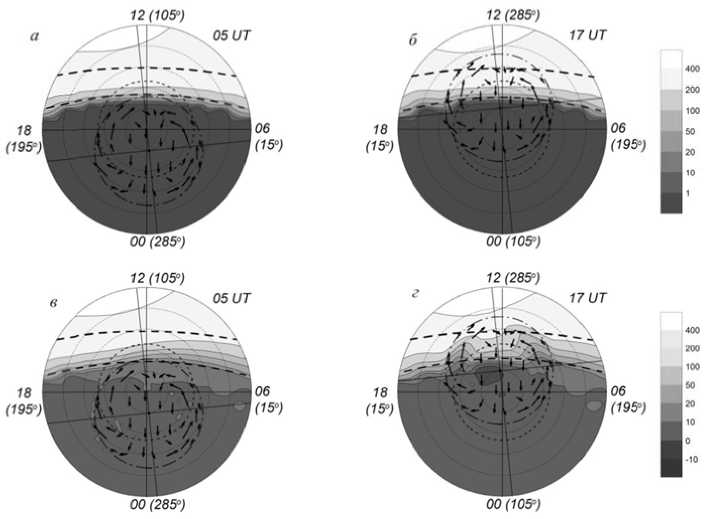
F igure 2. Distribution of the r a te of electron h eating by pho t oelectrons ( a , b ) and the elec t ron cooling ra t e ( c , d )

(eV ∙ cm–3 ∙ s–1) at 300 km at 05 and 17 UT

05 UT

05 UT

(13>)

06 (15-)

06 (15>)

05 UT

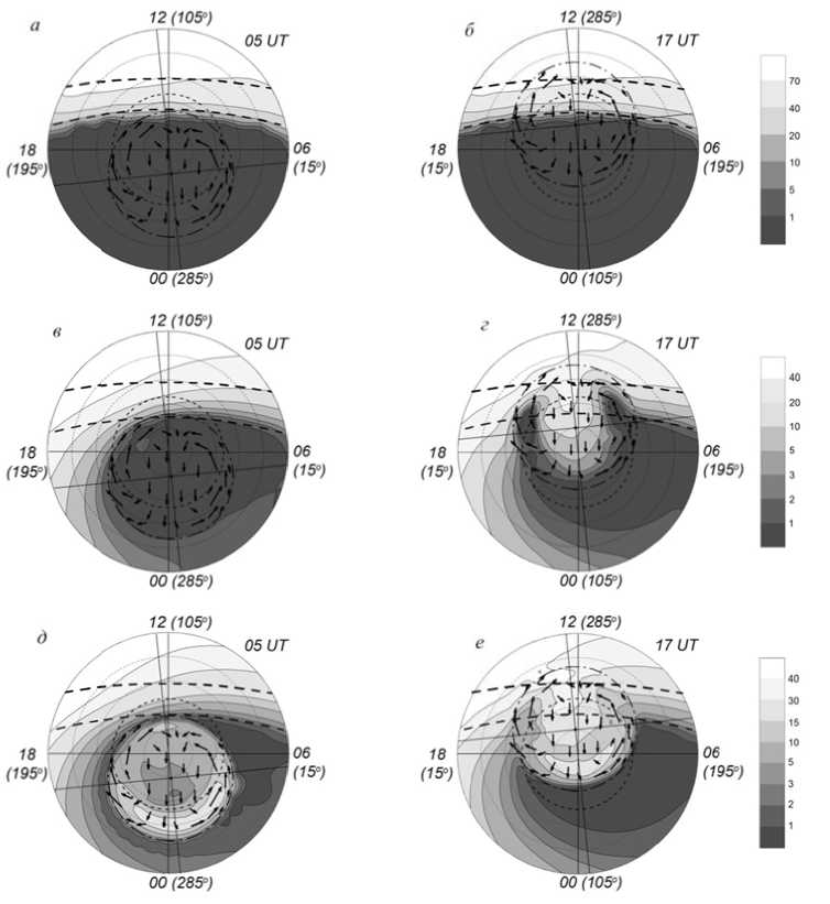
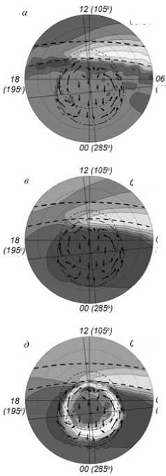
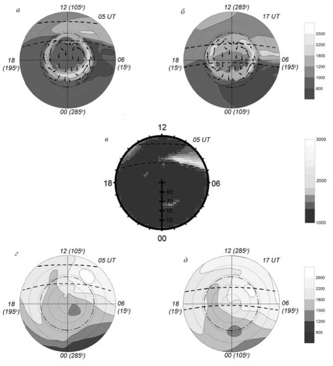
F igure 3. Distribution of the d i fference betw e en the electron gas heating and cooling rates ( a , b ) (eV ∙ c m ^–3 ∙ s^–1) and the electron temperature (K) a t 05 and 17 U T at 300 km, r e gardless of pr e cipitations ( c , d ) and with r e gard to them ( e , f )

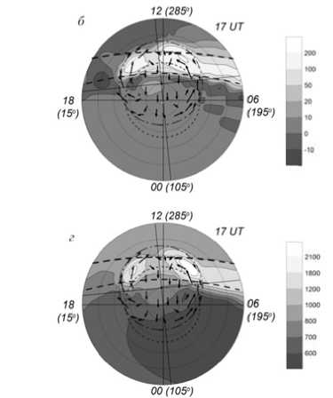
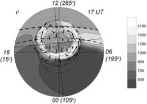
F igure 4. Electron temperat u re distributio n as deduced from the calcul a tion results o b tained by the model of the high-latitude ionosphere ( a , b ) at 400 k m , TDIM [Da v id et al., 201 1 ] at 400 and 8 00 km ( c ), a n d IRI-2012 ( d , e ) (K) at 400 km for 05 a n d 17 UT in g e omagnetic co o rdinates

F igure 3, a , b illustrates the calculated di s tribution of t he difference between elec t ron gas heati n g and cooling rates (or generalized rat e ) ∆ e = Q eλ – Σ L e and electron temperatu r e at 300 km a t 05 and 17 U T. As anticipated, at 05 UT the heatin g rate prevail s over the co o ling rate in t h e dawn sect o r, where Δ e r eaches values of 200 eV ∙ cm^–3 ∙ s^–1 and more. At U T 17, the sa m e values of Δ e are observ e d both in th e dawn and du sk sectors in troughs wit h low electro n density. Fig u re 3, c , d sh o ws that in th e dawn secto r in the area b etween the two positions o f the termin a tor, where Δ e grows, a zo n e of elevated T e develops. At UT 17, i n regions of trench-like tro u ghs (Figure 1 , d ) and in t h e zone between the positi o ns of the ter m inator with i ncreased Δ_e, electron tem p erature also r ises, exceedi n g 2000 K in “epicenters” o f the zone. P recipitatio n events cause T e to elevate on the nightt i me side (Fig u re 3, e , f ).

Figure 4 shows the results obtained with the model of the high-latitude ionosphere (a, b), the numerical model TDIM [David et al., 2011] (c), and the empirical model IRI-2012 [Bilitza, 2014, Truhlik et al., 2012] (d, e) at 05 and 17 UT. The calculations were made for winter conditions, average solar activity (F10.7 = 160) and low geomagnetic activity (Kp = 2) in the absence of heat fluxes from the plasmasphere. The terminator at a height of 400 km shifts northward of its first position by ~18°. Figure 4, d, e depicts both the terminator positions as in Figure 4, a, b. It is seen that in TDIM at 05 UT at 400 km in the dawn sector between the two positions of the terminator, as in Figure 4, a, a zone of elevated Te is formed. According to IRI-2012 data, at 05 UT the epicenter of the elevated Te zone in the dawn sector is located between the terminator positions outside the convection zone as in Figure 4 a, and at 17 UT inside it, as in Figure 4, b. This is consistent with the results of calculations by the model of the high-latitude ionosphere. In [Xiong et al., 2013, Truhlik et al., 2012], the IRI model is shown to poorly describe the distribution of ne and Te in the sub-auroral and high-latitude ionosphere of the Northern Hemisphere. This is probably responsible for the absence of the zone with elevated Te in the dusk sector at 17 UT. The qualitative agreement between the calculation results obtained with the three models allows us to state that the main causes for spatial and temporal distribution of electron temperature, which we discussed in this paper, are valid.

CONCLUSION

We have studied the spatial-temporal distribution of electron temperature in the F2 region of the high-latitude ionosphere, using numerical simulation and the three-dimensional model of the ionosphere, built on the basis of the Euler approach.

It has been shown that in the F2 region of the high-latitude ionosphere during minimum solar activity in winter solstice conditions, the mismatch between the poles leads to regular longitudinal features in the distribution of T e during Earth’s daily rotation: at 05 UT, when the Eastern Hemisphere is on the daytime side, a zone of elevated T e is formed only in the dawn sector; at 17 UT, when the Western Hemisphere is illuminated, in both the sectors. In this case, the mechanism of formation of these zones with elevated T _e is as follows: in the absence of a heat flux downflow in the dayside ionosphere in regions of electron density troughs, where the electron gas cooling rate is lower than that outside them, T e increases. This is consistent with [Schunk et al., 1986]. Further, we have demonstrated that causes of the formation of electron density troughs at different longitudes differ. So, at 05 UT, a trough near the terminator in the Eastern Hemisphere develops from the rapid attenuation of solar ionizing radiation at x>90° when the convection zone related to the geomagnetic pole is on the nighttime side. At UT 17, when this zone is partially illuminated in the Western Hemisphere, troughs are formed in the dawn and dusk sectors due to the transport of the weak nighttime ionization to the daytime side by convection, therefore at this moment of universal time we can expect formation of two zones of elevated T _e.

Finally, let us note that the numerical model of the high-latitude ionosphere described in this paper can be used to study its thermal regime, in particular, to examine causes of the formation of hot spots observable at heights of the F2 region.

This work was supported by RFBR grant No. 15-45-05090-r_vostok_a and 15-45-05066-r_vostok_a.